All posts by Rich

Da man... really...

Sonic Results for Commercial Instruments

In the last post, I provided the analysis results for the “C major scale” YouTube clip that I found. Here I will provide the results for the other two clips that I found and a couple of commercial instruments that I measured.

Sound Clips Found On the Web

I’ll start with the sound clips I found on the web.
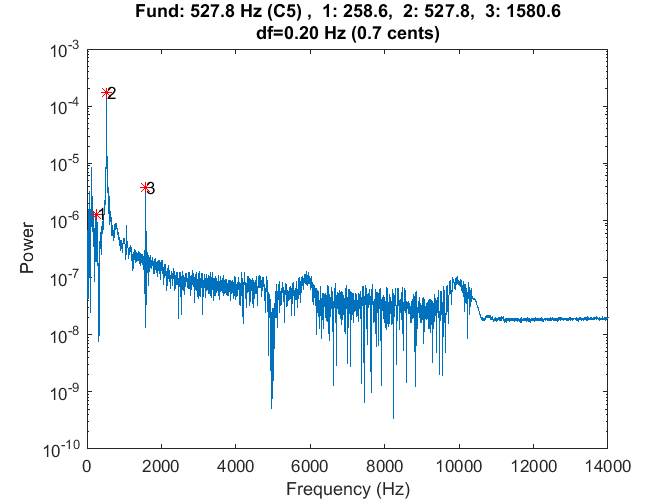
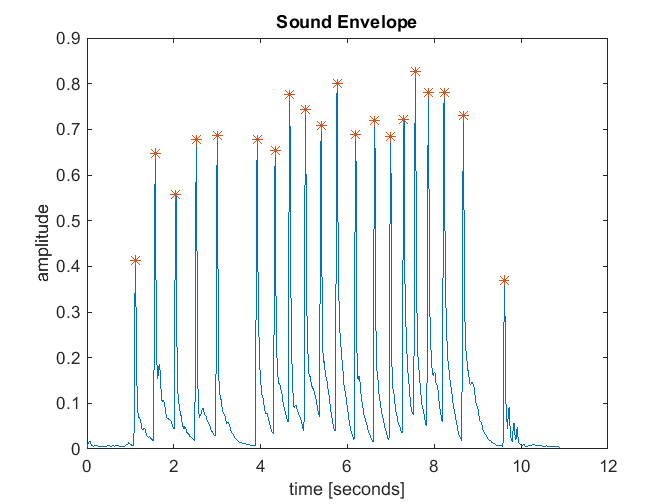
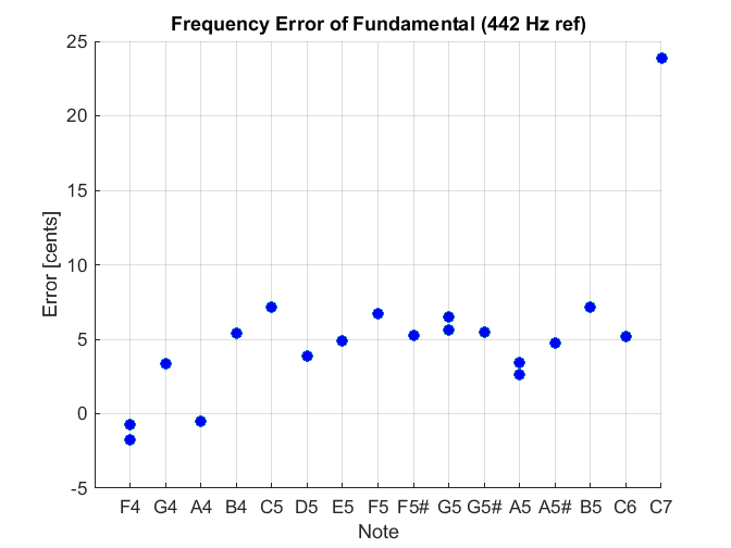
DeMorrow Results

Below are the two performance plots for the DeMorrow sound clip referred to in a previous post.

DeMorrow_envelope

DeMorrow_freq_errorDeMorrow_ratiosComments:

  • This instrument is in general a bit sharp with most of the notes in the range -2 to +7 cents.
  • A few of the notes were played twice. In that case the frequency error between the notes were within 1 cent, which was the desired resolution of the spectral analysis.
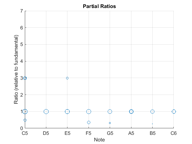
  • The notes in the lower register of this instrument had 3rd partials that were close to the desired ratio of 6. This is unusual as the 3rd partials for most instruments assessed tended to deviate from 6.

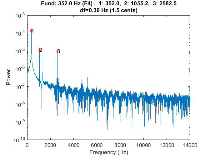
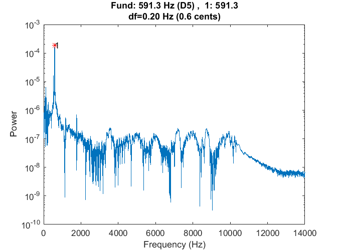
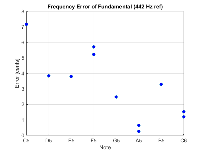
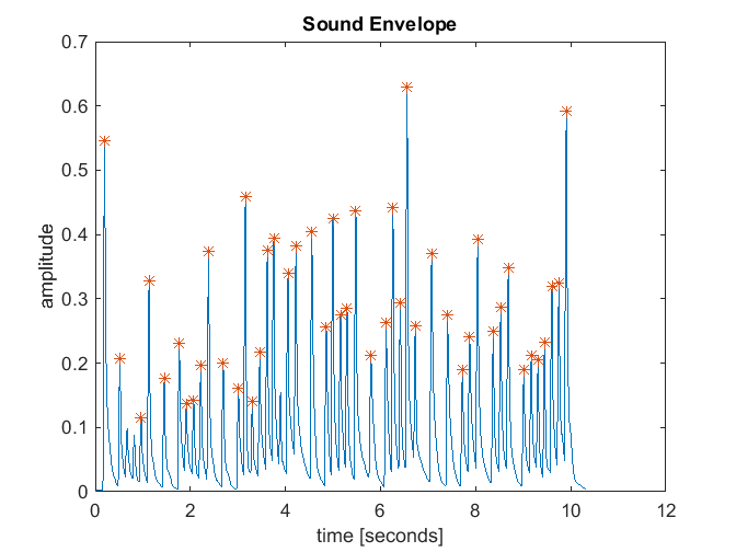
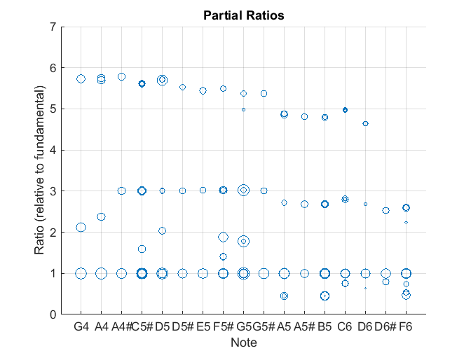
Oregon Symphony Results

Below are the performance plots for the instrument recorded on the Oregon Symphony website.
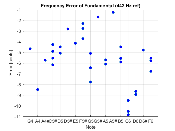
Oregon_envelopeOregon_freq_errorOregon_ratios

Comments:

  • The tempo for this sound file was pretty high, so that the notes were not allowed to decay completely. This resulted in generally short sound clips, which can result in poor spectral analysis results. This may be the reason for the somewhat unusual results observed for this instrument.
  • The 2nd partial ratios were generally good for the lower notes (below G5), but deviated from the desired value of 3 for the higher notes.
  • The ratios for the 3rd partial were all below 6, and generally trended lower with frequency.
  • The instrument tended to be a bit flat, and had fairly high variability of about +/- 5 cents (about the mean).

Measured Instruments

Because of the questionable quality of the web audio files, I also measured two commercial instruments myself. In addition to the improved audio quality, I was also able to control the cadence of the notes to ensure that the notes decayed completely.
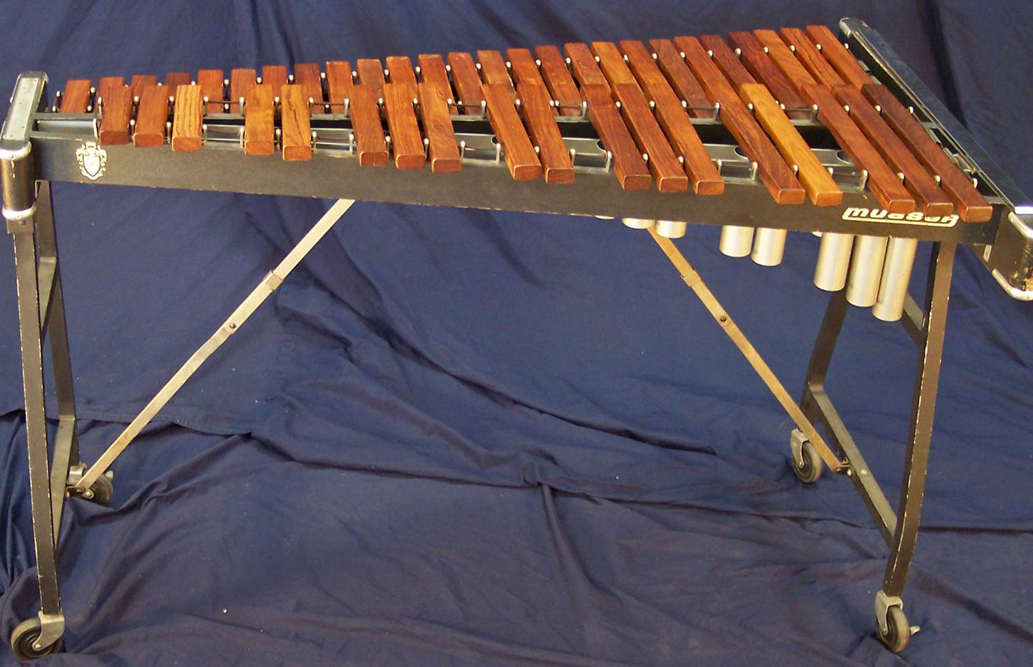
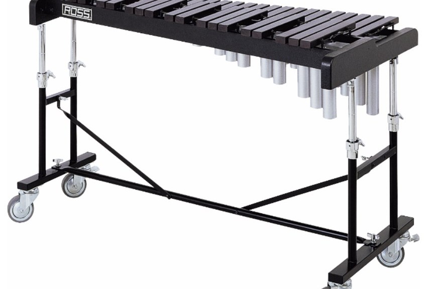
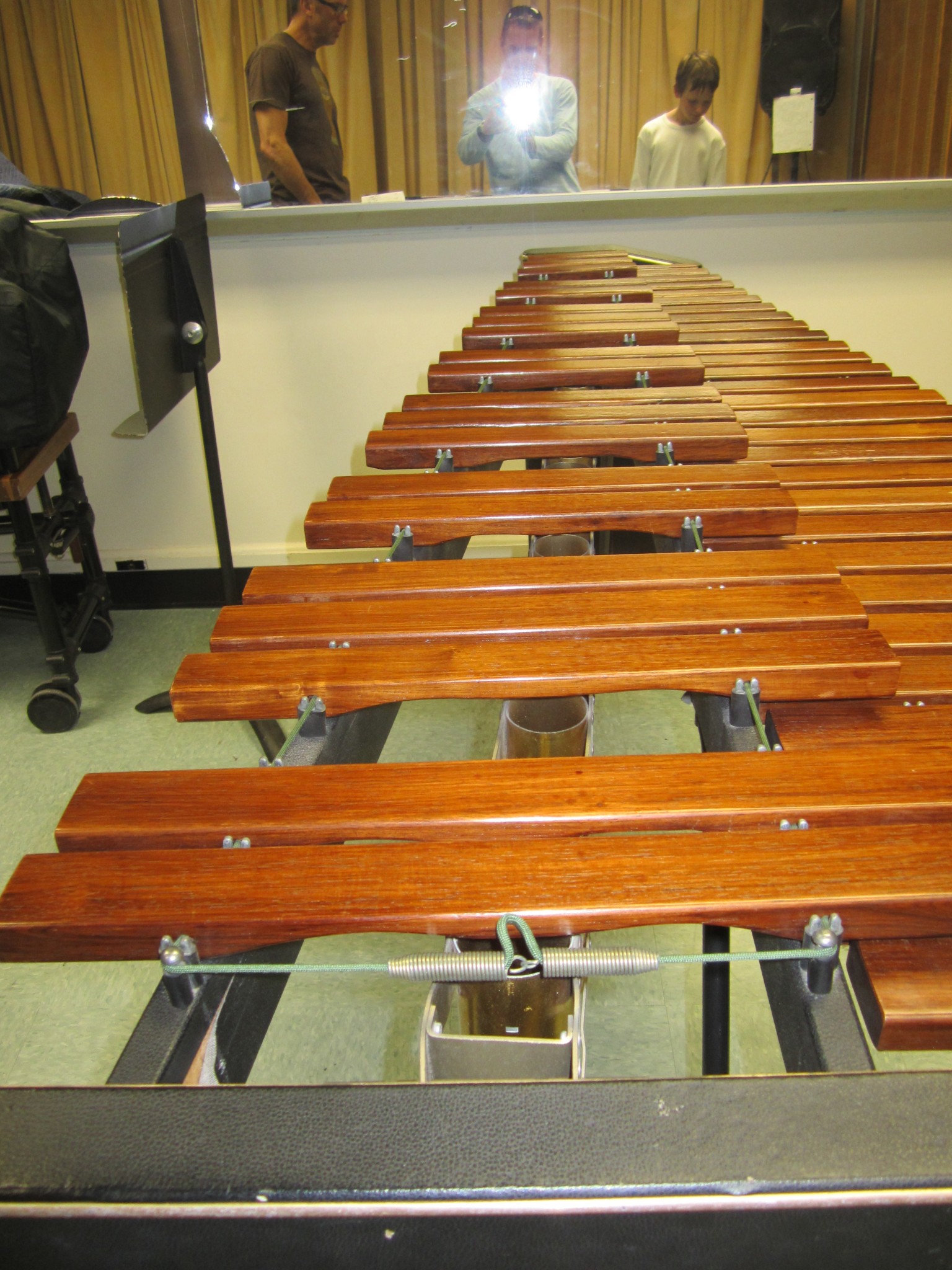
Ross R320 Xylophone

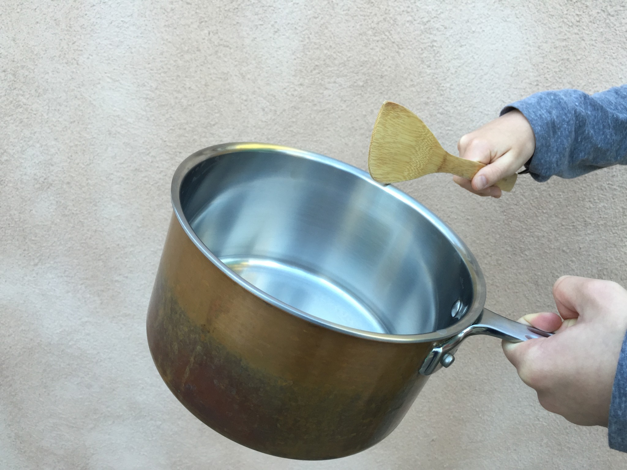
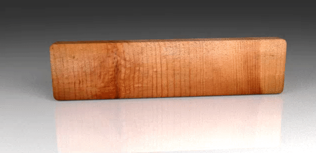
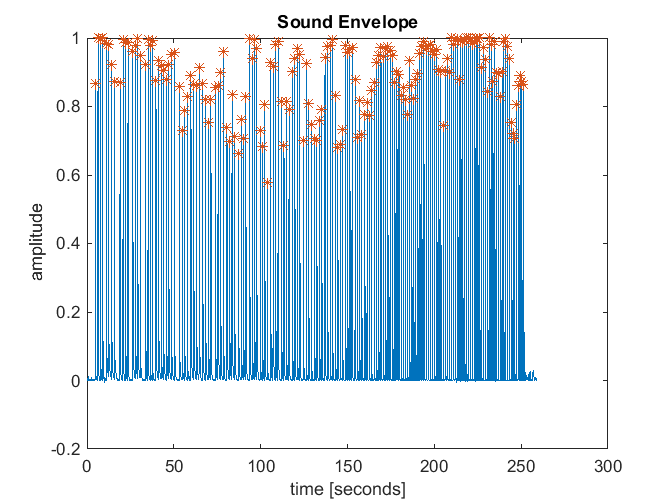
This is a xylophone that I measured at Jack’s middle school. His excellent band teacher, Mr. Sam Nesbitt, graciously provided access to the instrument and helped Jack and I obtain the recordings. This is a Kelon instrument which is pictured at the top of this post. When we recorded the instrument, we held the microphone about a foot above each bar, and struck each bar 4 times. Here is the sound file from that recording:

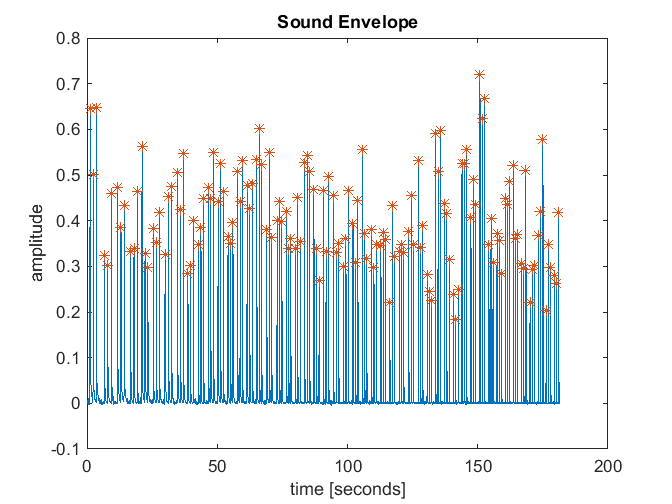
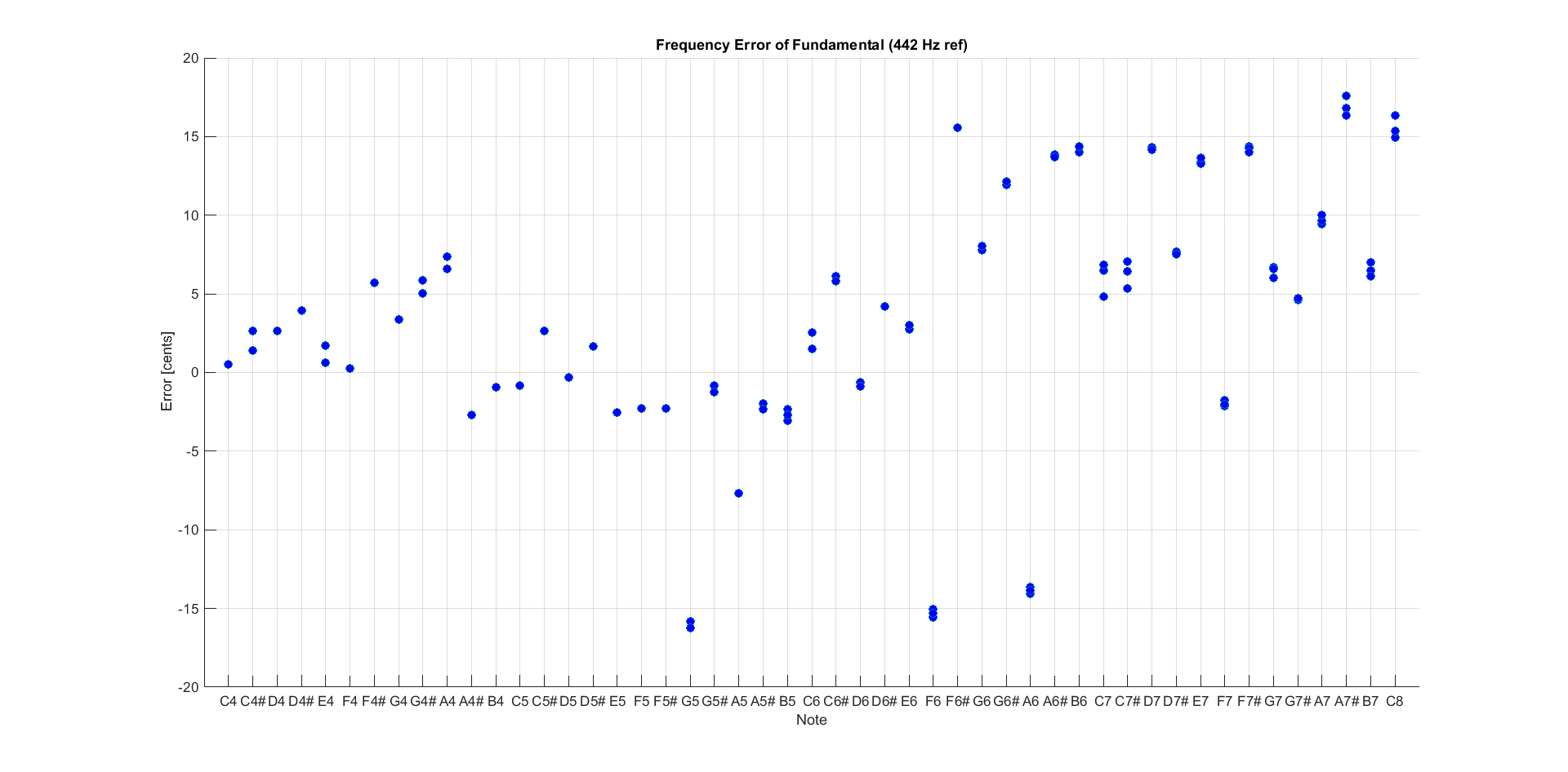
Here are the standard suite of performance graphs:

Ross_envelope Ross_ratiosRoss_freq_error

Comments:

  • As expected, the results from the spectral analysis are much better.
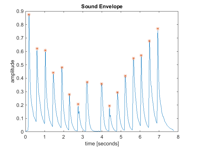
  • There were 176 discrete clips that were parsed, which is a result of each of 44 bars being struck 4 times.
  • For bars C5 and lower, the 2nd partial is spot on. The ratio for the bars in the higher register tended to be sharp.
  • No appreciable energy was detected in the 3rd partial. This may be because the bars were struck at their center point. If I were to record this again, I would strike the bars off-center; this tends to ring up more energy in the higher modes.
  • The tuning was quite good. In general, the instrument was only about 5 cents sharp, and the variance was very low; most notes were about +/- 2 cents about the mean.
  • The “clustering” of each group of 4 notes was very tight and only deviated by about 1 cent. This suggests the measured frequencies really are quite accurate.

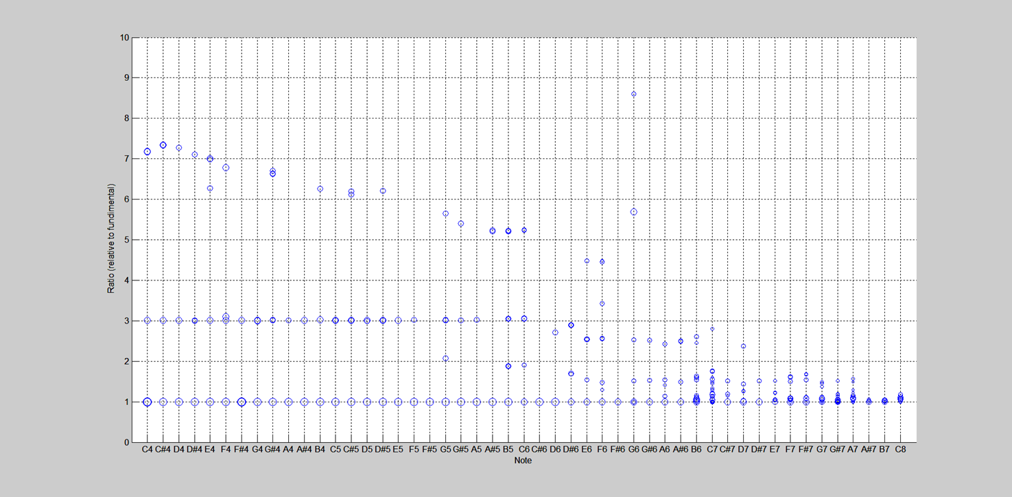
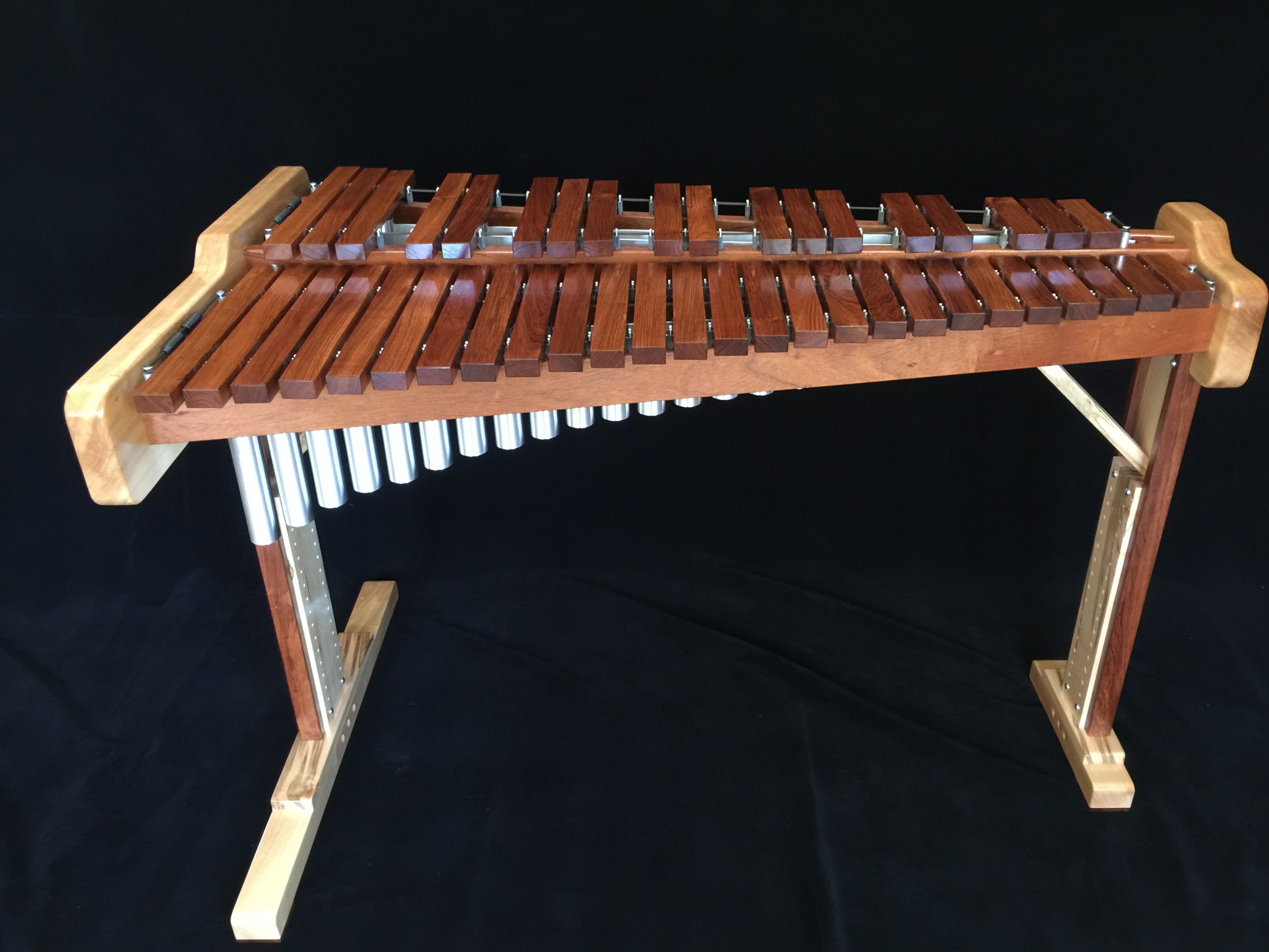
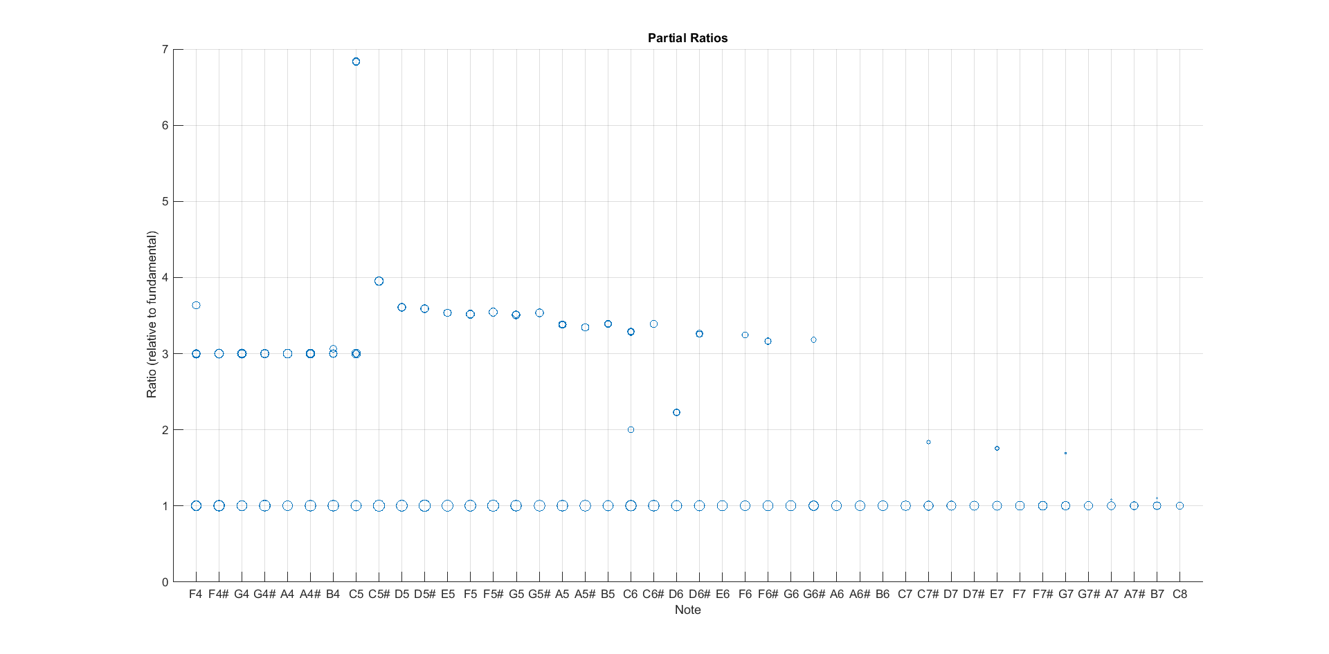
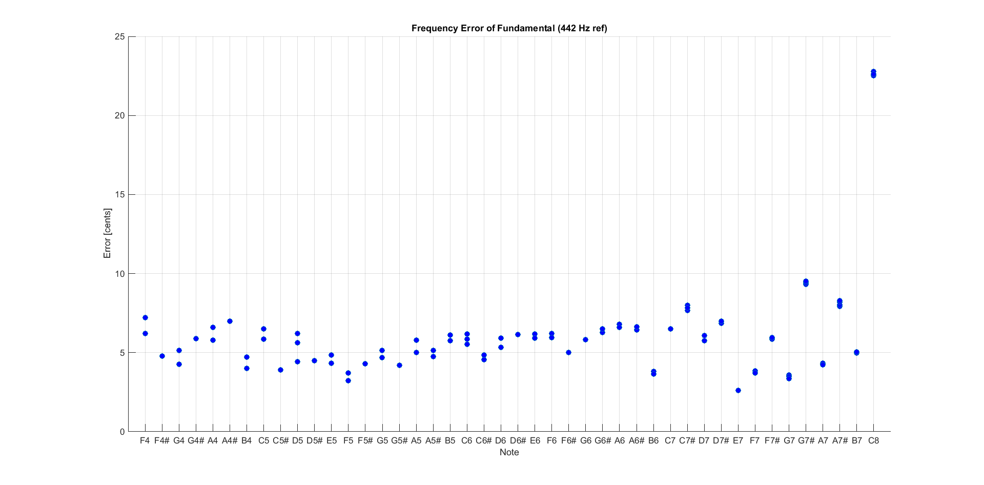
Kori Model 310 Xylophone

I went down to the University of New Mexico (UNM) to measure a second instrument. There, Jack and I met with Scott Ney, who is a percussion professor at the college. Scott graciously provided access to the Kori instrument and helped us make recordings. This was beautiful 4 octave xylophone with Honduras Rosewood bars.

Close up of Kori Rosewood bars.

Here is the sound file from that session:

The recording technique was similar to the other, but this time, we struck each bar three times.

Here are the standard performance graphs:

Kori_envelope Kori_ratiosKori_freq_errorComments:

  • This recording had 147 discrete clips that resulted from striking 49 bars 3 times each.
  • The 2nd partials were pretty consistent at 3 until about C6, when they started to go flat. This suggests that it may not be possible to accurately tune the 2nd partials for the shorter bars.
  • The 3rd partials were present, but the ratios wandered from >7 to less than six as the fundamental frequencies increased.
  • The mean tuning of this instrument was very good, but the variance across the bars was large with a pk-pk error of about +/- 15 cents. (However, the spread was much smaller in the lower register, where the ear is most sensitive.) Scott said that the instrument was definitely due to be tuned, which was apparent from the results.

My Take-Aways

I learned a lot from the web clips that I found, but the fidelity of the clips makes me question the utility of the data. I found the results from the two instruments that we recorded to be much more reliable. In bullet form, here are my most important findings from this effort:

  • Most of the instruments did a good job of accurately placing the 2nd partial at a ratio of 3. I concluded that carefully tuning this mode is both achievable and important. However, it may not be possible to accurately tune the 2nd partial for the shorter bars.
  • The 3rd partial was not reliable across the instruments. Only the DeMorrow achieve 3rd partial ratios that were close to 6, and that was only for the bottom bars. This finding, plus challenges in designing a bar with reliable 3rd partials (which you will here more about later,) suggested that I should not obsess over tuning this mode.
  • In general, trying to obtain good absolute tuning is desirable and achievable, but even instruments with fairly large frequency variance sounded good. Based on the findings, I decided to shoot for tuning accuracy of 2 or 3 cents.

OK. Now I knew how accurate the bars must be tuned. In my next post I will begin to discuss how to determine the bar shapes.


Spectral Analysis and Performance Plots

As noted in the last post, I was only able to find 3 recordings of xylophones on the web that were suitable for spectral analysis. I also described some software that I wrote that spectrally analyzes the clips. In this post, I will discuss some practical implications of the spectral analysis and will discuss some “standard” plots that I use to summarize xylophone sonic performance.

Performance Analysis

We will start with the first sound clip – the c-major scale video example. Below are some plots produced by the Matlab scripts. You will see a lot of these, so I will take a moment to explain each.

Sound Envelope Plot

The plot below shows the sound envelope for the YouTube C major video clip.

Sound envelope for "C major scale" web video
Sound envelope for “C major scale” web video

The envelope of the sound clip is basically a curve that contains the amplitude of the sound over time. The example above is typical in that each bar strike produces a sharp peak followed by a decay in the sound amplitude. This information is used to break apart the single sound file into a set of discrete clips that can be individually analyzed. If you count the peaks in this example, you can see that 16 discrete notes were played. This is because the guy played up, and then down the C major scale – he played C, D, E, F, G, A, B, C, C, B, A, G, F, E, D, C.

Spectral Analysis

Once each note is separated out of the sound file, the data can be analyzed to determine the spectral content. A full description of spectral analysis is way beyond the scope of this blog, but there is plenty of information on the web. The basic idea is to analyze the sound bite to determine the power at each frequency. If done carefully, this will show peaks at the resonant modes of the bar. The magnitude of the peak represents the power in each resonant mode, and the location of the peak determines the frequency. By analyzing the series of peaks produced, it is possible to determine how well the bar is tuned.

Well, that is the theory; in practice, it gets a bit more complicated for a few reasons. First, the duration of each note is short. This complicates the spectral analysis somewhat. Specifically, short transient clips can result in spectral leakage and poor frequency resolution. I used a very standard Fast Fourier Transform (FFT) based spectral analysis technique. To address the spectral leakage problem, I sometimes  windowed the sound clip prior to applying the transform. To address the frequency resolution problem, I zero-padded the data to increase the length of the clip. This tends to reduce the signal-to-noise (SNR) ratio of the clip, but allowed a more precise determination of the frequency of each mode to be made.

Another difficulty of bar tuning by using spectral analysis is related to the nature of wood itself; wood is only approximately homogeneous as its density varies throughout due to internal checks and knots. This variability can result in extraneous resonant modes that are identified by the spectral analysis. For example, consider the spectral plot at the top of this page. The software did a good job of identifying the first three partials and labeled them 1, 2 and 3. However, there also exists a mode just to the right of the second partial. This is real, and can affect the tonal characteristics of the bar.  These extra modes can sometimes confuse the software and make the plots a little messy, especially when producing “roll-up” plots that provide data for all notes. For example, here is plot showing the ratios of the partials that were determined by analyzing each note of the C major scale clip form the YouTube video:

Ratio of measured partials for each note.

On this “ratio plot,” the note names are plotted along the abscissa, and the ratios of the measured partials are plotted along the ordinate. The note names are determined by finding the closest ideal note (based on a 442 Hz pitch reference) to each measured fundamental frequency. All data for a single note are plotted in the “column” above the note name, so if a particular note is contained multiple times in a sound file, this will result in little groups of points that are close together. The circle size on the plots relates to the power in the partial. (Actually, the size is proportional to the log of the power.) Typically, the larger circles represent modes that we care about, and the smaller circles correspond to low power extraneous modes that don’t affect the sound too much.

Spectral Analysis Challenges

You will notice some weirdness in these plots from time to time. As noted above, this is typically due to extraneous modes. For example, consider the first note from the C major sound clip. Here is the FFT for that note:

First note of C major sound clip.

The software correctly identifies the two dominant modes, labeled 2 and 3 on the plot above, but it also finds another tiny mode that is below the fundamental frequency of the note. This may be real, it may be some artifact of the spectral analysis or it may be the result of poor sound fidelity in the YouTube clip. In any case, the result is the extra circle on the plot that has a ratio of about 0.5. In some cases, extra tones will appear that result from torsional modes in the bar (as described in LaFavre et al,) especially if the bar is not struck at the bar center.  The good news is that the software still correctly identified the fundamental (i.e., the major peak at 527.8 Hz) so that the ratios can be calculated correctly.

In addition to the extraneous modes, the other oddity that the the ratio plots will sometimes exhibit is missing modes. For example, in the ratio plot above, the software did not find a second mode for most of the notes. Here is the FFT for the first D5 note in the sound file:

FFT for the first D5 note in C major sound file.

The fundamental mode is easy to identify, but then there are some very small peaks later on in the plot that may or may not correspond to the second partial. The lack of significant peaks for the higher partials may be the result of the poor sound file quality, or it may be the result of where the bar was struck – I found that when the bar was struck “dead center,” the second mode was typically very weak and difficult to measure. You will here lots more about this later when I get into the discussion on bar tuning.

The “ratio plots,” like the one shown above, are useful because they quantify how well the instrument produces partials in the desired 1:3:6 tuning ratio. However, the ratios are normalized to the measured fundamental, so they do not quantify the absolute tuning accuracy of the instrument. Consequently, I produce a plot of the tuning accuracy for the fundamental mode like that shown here (again, for the C major sound file):

Absolute frequency error for fundamentals of C major scale sound file.

This “absolute tuning error” plot quantifies the error, in cents, for the fundamental frequency of each note. In musical parlance, the space between adjacent notes on an equally tempered chromatic scale can be broken up into 100 equally spaced intervals. Each of these intervals is called a “cent.” Mathematically, as previously noted, the interval between notes is given by the ratio 2^(1/12) ~= 1.0595. A cent is defined as the interval 2^(1/1200) ~= 1.000578. Because a cent is defined as a frequency ratio, the frequency interval corresponding to a cent varies with frequency. For example, a cent for the C5 note corresponds to a frequency delta of

FreqDelta = Freq_C5 * (1-2^(1/1200)) = 525.63 * 0.000578 = 0.304 Hz

In contrast, the frequency delta of a cent for the D5 note is 0.341 Hz.

The absolute tuning error plot presented above shows that the xylophone used to produce the C major sound clip was tuned a bit sharp for all of the notes of the scale. The C5 note was worse, at about 7 cents sharp. The A5 note, however, was almost spot on.

Finally, the Results

The above description is a bit verbose, but it is necessary to understand the results of the analysis for the various xylophones that were analyzed. The results of these analyses motivated the tuning approach of my own xylophone bars and I believe provide a unique and practical reference for those interested in quantifying the sonic performance of xylophones. In the next section, I will present the actual results of these analyses.

Analyzing Xylophone Sound Clips Found On the Web

As the previous posts note, the desired frequency ratios for the first 3 partials of a xylophone are 1:3:6.  However, I needed to know how accurate these frequencies had to be to yield a nice-sounding instrument. I couldn’t find comments on the web about the tuning accuracy requirements, so I set out to spectrally measure some instruments to serve as a guidepost. Specifically, I needed to know how accurate I needed to tune the fundamental and higher partials.

Finding Sound Samples On the Web

The web was pretty skimpy when it came finding sound clips of xylophones.

Here was the first clip that I found – basically a guy playing a C-major scale. There was no info on the type of xylophone he was playing, but it looked pretty decent.

Here is another video that I found of a DeMarrow instrument. He hits some notes at the end of the video.

Finally, at  this site I found a third clip of a guy from the Oregon Symphony playing an xylophone. Again, the I couldn’t find the xylophone brand, but decided it must be a good one if it is used in the symphony.

Spectral Analysis

So here is where the magic starts – I wrote some software in Matlab that analyzes these clips to determine how accurately tuned the xylophone is. The tool, called AnalyzeClip, performs the following steps:

  1. Read the WAV file.
  2. Delineate  each discrete note (i.e., each time a bar is struck) into its own clip.
  3. For each clip, perform a windowed spectral analysis.
  4. Find the peaks in the spectrum (aka, the modes). This identifies the frequencies associated with the fundamental frequency and the higher partials.
  5. Find the fundamental. This is the lowest mode and typically has the most power (although not always – sometimes I found that the second partial had more power.)
  6. Associate the fundamental with the closest ideal note, assuming an equal-tempered scale with a 442 Hz reference pitch (Wikipedia has a nice description of equal temperament.)
  7. Compute the frequency error of the fundamental relative to the ideal desired pitch.

The “ideal pitch” noted in the last step is computed for a an equal tempered scale with a 442 Hz reference. The notes in an equal tempered scale have a ratio that is given by 2^(1/12) power, which is about 1.0595. So if you want to determine the frequencies associated with a note, just multiple the previous notes frequency by 1.0595. If you do this multiplication for 12 successive notes, the two bookending notes will have a ration of 2, or an octave apart. For my 3.5 octave xylophone, the following table gives the desired frequency for each note.

Note frequencies

Bar NumberNoteFrequency
1F4350.816
2F#4371.676
3G4393.777
4G#4417.192
5A4442.000
6A#4468.283
7B4496.128
8C5525.630
9C#5556.885
10D5589.999
11D#5625.082
12E5662.252
13F5701.631
14F#5743.352
15G5787.554
16G#5834.385
17A5884.000
18A#5936.565
19B5992.256
20C61051.259
21C#61113.770
22D61179.998
23D#61250.165
24E61324.503
25F61403.263
26F#61486.705
27G61575.109
28G#61668.770
29A61768.000
30A#61873.131
31B61984.513
32C72102.518
33C#72227.540
34D72359.997
35D#72500.330
36E72649.007
37F72806.525
38F#72973.410
39G73150.218
40G#73337.540
41A73536.000
42A#73746.262
43B73969.026
44C84205.036

Notice that bar 5 (A4) has a pitch of exactly 442.00 Hz. This is because I referenced all of the other notes to this pitch.

In my next post, I will show some results form the spectral analysis of the sound bites that I found on the web.

Checking Out the Competition

Having never played a xylophone (or even seen one up close) I decided my first step was to check some out – first on the web, and the up close and personal.

Typical Characteristics of Commercial Instruments

I found a lot of pictures on the web of commercial instruments made by Musser, Malletech, Deagan, Yamaha, etc. that I used to sort of check out the least common denominators. Most concert instruments were 3.5 octaves, which means they had 44 bars that typically spanned the range F4-C8. This range seemed to be most common, so I decided to use it to baseline my design. I also discovered that that there are basically two tunings: The A4 bar can either be tuned to a frequency of 440 Hz or 442 Hz. The literature suggested that 442 tended to sound brighter with an orchestra and is more common, so I decided to tune mine to that frequency.

Bar Materials

I also saw that there were at least three bar materials that were common. The first is a synthetic called Kelon. I’m not sure exactly what Kelon is, but it kind of feels like fiberglass. The advantage of Kelon is that it is cost effective and doesn’t change tune with humidity and temperature. Here’s a link to a pretty nice Musser xylo made of Kelon.  Through my research, it appeared that Kelon is primarily used for instruments that see a lot of travel and abuse (e.g. schools).

I also saw a lot of instruments made of an exotic hardwood called Padauk. Here is a link to a Yamaha xylophone made of Padauk. It appeared that instruments made of Padauk were more expensive than those with Kelon, yet less expensive than those built with Honduras Rosewood, which is the traditional wood used to build xylophones and marimbas.

Ah Honduras Rosewood…the holy grail of xylophone woods (cue angel chorus and sunbeams). As you move up the xylophone food chain, pretty much all of the high-quality instruments are made of Honduras Rosewood. It turns out that this wood is unique in its properties relative to making idiophones (Remember? Instruments that you whack.) If you check out the paper by Aramaki cited below, you can see that they build bars from 59 species of wood. Which one came out on top? You guessed it, Honduras Rosewood.

Dimensions

OK, so after a little research, I had settled on a note range, a tuning pitch, and a  bar material. The only basic characteristic left to decide  was size. If you troll around the web, you can see that bar sizes vary quite a bit. For example, from the LaFavre site, I found the dimensions of the F4 bar (the longest bar) on a Deagan was 12.81 x 1.93 x 0.95 inches. However, the F4 from a the Kori instrument I measured was almost 17 inches long. These tended to be the extremes I found, and most other instruments had bar lengths within this range. As we will see later, a wide range of bar lengths can be shaped to yield the desired frequencies. From a physics standpoint, the larger bars will produce more more volume, as they have more surface area that is creating sound. However, this greater amplitude comes at the expense of compactness and portability.

In the end, I modeled the dimensions of my instrument off of a rosewood Yamaha instrument that seemed to be popular. The specific instrument is a Yamaha YX-500R and can be found at this site.  I liked the overall dimensions of the Yamaha, as my instrument has to fit in my house. Best of all, I was able to find a exploded diagram with parts list on the Yamaha site! Here is one of the diagrams.

YX-500R_exploded
Exploded diagram for Yahama YX-500R

and here is a section of the parts list.

YX-500R_bar_length
Partial parts list for Yahama YX-500R

The bar description has the length and width of the bars. Sweet! The longest bar on this instrument is 380 x 38 mm which is about 15 x 1.5 inches, which is right in the middle of the range of most of the xylos I found. Also, by following the dimensions of the Yamaha instrument, I was able to ensure that I would build a xylophone that was 1) about the size expected by a musician and 2) had bar lengths that were guaranteed to be tunable.

Next Up

In this discussion, I focused mostly on the physical attributes of the commercial instruments that I found. In my next post I will dig in to the sound characteristics, including more than you probably want to hear about the spectral analysis software I wrote, and the results from a few instruments I analyzed.

References

Aramaki et al. 2007: Aramaki, M., Baille`res, H.,Brancheriau, L., Kronland-Martinet, R., and Ystad, S.(2007). “Sound quality assessment of wood for xylophone bars”, J. Acoust. Soc. Am. 121, 2407–2421.


A Little Background

OK, we’re getting smarter. We now know that it is necessary to shape the underside of the bars to tune them; this is a good start!

“But what is the right shape?” An even more fundamental question is, “What are the desired frequency characteristics for each xylophone bar?”

Before anything else, I want you to know that I am not a musician; I have dabbled in guitar and ukulele, but my instruments mostly just collect dust in my closet nowadays. My point is that while I’ve got a decent handle on the engineering and science, I am less than an expert on the musical implications of xylophone tuning. So for the musical purists out there, please cut me some slack.

One very important fact about xylophone bar tuning is that it is necessary to control the fundamental and overtone frequencies in order to make a harmonious bar. Tones produced by the bar should produce a chord, rather than a series of unrelated sounds. Note that the term “partials” is used to describe the various tones produced by the bar. The first partial (the lowest, and most dominant tone) is called the fundamental, and the higher partials are often called the overtones. To clarify:

fundamental = first partial

second partial = first overtone

third partial = second overtone

And so on…

A Semantic Warning!

There seems to be some overloading of the term “partial” in the literature. It appears that the engineers use the term differently than the musicians. For example, the Bork paper defines the term “partial” to be any of the dominant tones produced by the bar (consistent with my use above). These might be frequencies that are integral multiples of the fundamental, or they might not be. However, in the musical literature, it appears that the term is often used to describe the integral harmonic. For an example, check out this informative site from the Vienna Symphonic Library. In that post they state, “Xylophone bars are often tuned in such a way that the 3rd partial (= octave + a fifth above the pitch of the fundamental) is more prominent, …” An octave plus a fifth corresponds to the frequency ratio of 3, relative to the fundamental. So when they say the “3rd partial” they are referring to the tone that has a frequency of 3*fundamental. However, this is the second dominant tone, so Bork and I would call that the 2nd partial. I am not sure what the “correct” use is, but be aware of this confusion and note that I will use the Bork definition consistently.

More Semantics…

Sometimes the term harmonic is also used. Harmonics are partials that are integral multiples of the fundamental frequency. That is, they are frequencies that are like 2*f, 3*f, etc., where ‘f’ is the fundamental frequency. Values like 2.153*f or 5.416*f are not harmonics because they are not integral multiples (i.e., they are not whole numbers times the fundamental). Lots of folks incorrectly use the terms harmonic to mean any frequency higher than the fundamental.  I am guilty of this semantic misuse too, but will try to use the proper term partial to avoid confusion. See Wikipedia for a much more careful description of these terms.

Semantics aside, here is the important part: for a xylophone bar to sound good, the ratios between the first two overtones, relative to the fundamental, must be specific values. Namely, in the United States, the bars are tuned so that the ratios are 3 and 6. That is, the second partial has a frequency of 3 times the fundamental (i.e., first partial), and third partial has a ratio of 6 times the fundamental.  In shorthand, the ratios are 1:3:6. This is sometimes called “quint” tuning because the second partial is a major fifth above an octave. You can learn a little more about quint tuning at the Deagan ebsite.

Without getting too far ahead of myself, here is a chart that provides the tuning of the first 3 partials for the Kori xylophone at UNM.

Measured spectral tuning graph for Kori xylophone.

On the graph, the notes are plotted along the bottom, and the frequency ratios for the measured partials are plotted on the y axis. Clearly, the first and second partials are right on the money (at least for the lower notes). Third partial, however, sort of wanders around the desired ratio of 6. You will hear lots more about my spectral analyses of various instruments later.

Why 1:3:6?

It is reasonable inquire about the origin of the 1:3:6 tuning ratio. To be honest, I didn’t find any great explanations of this, but there is some good literature on the web that describes why certain tones sound good together. For example, check out “The Physics of Music and Musical Instruments,” which has all kinds of good info. Alsocheck out “The Art and Science of Mallet Instrument Tuning,” which has an excellent discussion of some history of tuning and some discussion of the rationale for quint tuning.

In the next post, I will start to get into the approach to determining the correct bar shape.

REFERENCES

[1] I. Bork, “Practical Tuning of Xylophone Bars and Resonators”, Applied Acoustics 46, 103-127 (1995).

It’s all about the shape

It didn’t take a ton of research to figure out that the xylophone bars had to be shaped, not just cut to length. In this case, tuning means carving the bottom of the bar to yield the desired tonal characteristics.

Here is a picture of the underside of the bars for a Kori xylophone that I checked out at the University of New Mexico. Thanks to Scott Ney, I was able to dissect this instrument!

Shaped underside of some of the bars for a Kori Model 310 xylophone.

While I don’t have the skill (or patience) to provide a full-on description of the physics related to vibrating objects (like a xylophone bar,) I will describe a few basics to get you started. Nerds: you probably already know this stuff and can safely skip to the next section.

Vibrating Bodies

We all know that when something, like a bar of wood, is whacked, it vibrates for a while and then the sound eventually dies out. The duration of the sound is referred to as the “decay” of the signal, and there is a precise definition that quantifies the decay duration in seconds. What many people don’t know is that pretty much every object has a preferred frequency at which it generally vibrates. Think of whacking a frying pan versus big pot; you can hear the difference in the tones between these two objects. The frying pan “wants” to vibrate at a higher frequency than the big pot. Further, each object will typically vibrate at a series of discrete frequencies called modes.

For those without science knowledge, what you may not know is  that what you are really hearing is one “fundamental” tone, and then a series of different, higher tones that are related to the fundamental tone in complex ways. It is the relationship of this fundamental tone and the “overtones” (and how quickly each tone dies off) that creates the overall tonal characteristics (i.e., the timbre) of the object.

It turns out that it is possible, by choosing the shape of the object, to control the fundamental and overtones.

WARNING: You’re entering a zone of extreme nerdiness. If you don’t care about physics and math, you may want to skip the next few sections. Although, be warned – nerd-speak is sprinkled throughout  the rest of this blog.

nerdvenndiagram
Helpful diagram to determine if you are a nerd.


Building a xylophone in 613 easy steps

Our xylo-adventure started when Jack asked for a xylophone for Christmas. He wasn’t asking for a Fisher Price, but rather a full-on concert grade instrument.

Not the xylophone Jack wanted.
Not the xylophone Jack wanted for Christmas

Jack plays piano and percussion in his school bands and wanted an instrument to practice at home. My knee-jerk response was to say “sure, dude!”  When I did my research, however, I almost had a heart attack- I was not going to pay $2000-$4000 for a series of wooden blocks! So I, an electrical engineer and a weekend woodworker, set out to build one. “How hard could it possibly be to build a one?” I asked myself. (Answer: pretty damn hard!)

So last December, I jumped in with both feet. Like most people, I assumed that Google would do the majority of the work for me. Over  Christmas break, I begin scouring the web. My laptop kept me warm for countless winter evenings while I searched for a canned xylophone recipe. It quickly became apparent that if anyone like me had built a high-end xylophone, they had not published their efforts on the web. I found lots of “toy” efforts built from PVC pipe and the likes, but got exactly zero hits on building a concert xylophone. Along the way, I did find one amazing site called La Favre that had tons of info about building a marimba (basically a giant xylophone). The La Favre site was pivotal in that it was the first source that I found that addressed tuning of the bars. It doesn’t take more than high school physics to know that the longer the bar, the lower the pitch; I, therefore, assumed that tuning just meant cutting the bars to the correct length. Au contraire – the tuning of idiophone bars (the fancy, scientific name for musical instruments that you whack with a stick) is performed by shaping the underside of the bars in just the right way.

One of my "shaped" xylophone bars.
One of my “shaped” xylophone bars.

Getting shape right is really the secret sauce to building an instrument that sounds great. Stick with me and you’ll hear a lot more about this!

A Teaser…

As a teaser, below is a one-page summary of the xylophone that Jack and I built. Read the subsequent posts if you want to learn more about our journey.

The whole project distilled into a single page

Here is what it sounds like. These are just a couple of clips of Jack noodling around.

Here is a photo of the completed instrument.

The final product!
The final product!

May 21, 2016 update: Here is a sound file of Jack playing a song he learned. The recording is so-so, but hey, I’m not a recording engineer!

First post – and introductions…

Bear with us – blogging is entirely new to our family; we’re totally just groping around in the dark! Despite our inexperience, we are going to give this the old college try. So here goes…

About Us

I guess introductions are in order. My name is Rich Wickstrom, and this is a site that I’ve created for my family and me.

Rich in his natural habitat (in the garage smoking a cigar)


The actual catalyst for creating this site was the completion of a xylophone that my son, Jack, and I built. I’ve always taken advantage of the vast information available on the internet. I am, however, guilty of not really giving back. Our xylophone project was extremely unique but had a very limited audience. It seemed to me, however, that maybe,just maybe, there was at least one person out there who could make use of my highly-specific information. But before jumping in to the xylophone project, let me take a moment to introduce my family.

Here’s we are:

IMG_0472
Powerpuff Girls (feat. Hit Girl)

From left to right, that’s Jack, Rich, Lily and Lynette.

We don’t always dress up as cartoon superheros. Here’s a photo to prove it:

The family
The fam

Our Site Name

Oh yeah, why supermediocre.org?

One day, my daughter, Lily, and I were brainstorming name ideas; we were gravitating towards names that were quirky and sort of self-deprecating. The mashup “super mediocre” eventually came up. We liked that it was an oxymoron and sort of off-balance; it fit our family in some twisted way.  I checked if the domain was available – it was (big shocker).

In the end, we thought the name supermediocre was, um…perfectly OK.