With the rough tuning done, and the holes drilled, Jack and I moved on to the fine tuning. Our goal going in was to get the fundamentals to within about 5 cents.
The fine tuning took a bit more time than the rough tuning, because we had to be very careful not to remove too much wood – you really have to sneak up on the target frequencies.
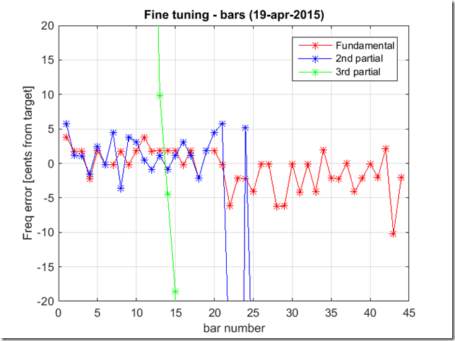
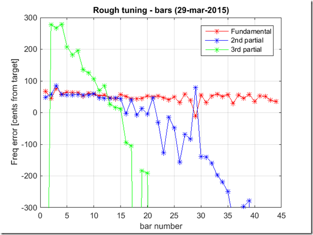
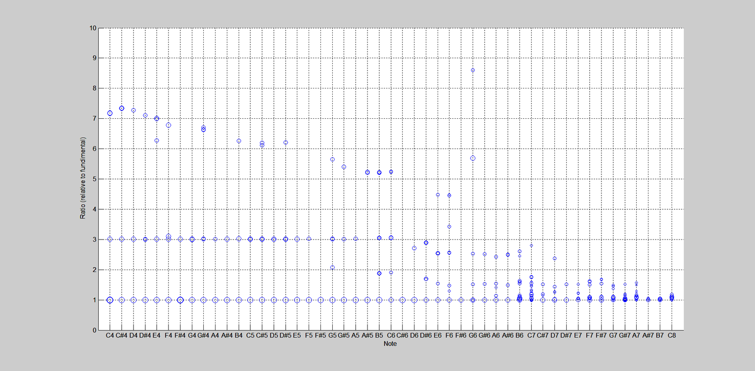
After all of the iterations, here is a plot of the resulting bar frequencies and overtones:
Bar frequencies after final tuning
As you can see, the fundamental frequencies are almost all within +/- 5 cents. For bars 21 (C#6) and under, we were able to keep the second partial pretty tight too. We were not able to maintain the 2nd partial in the higher register, but this is consistent with other instruments that I spectrally measured. We expected the bars to settle out a bit more, so our plan was to tweak them one last time before applying finish to tease out the last few cents.
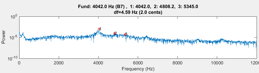
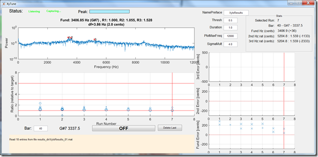
Bar #43 (B7) was problematic. As we were tuning it, it sounded a bit dead. The spectral response looked a little funny too. Here is the PSD for that bar:
Bar 43 PSD
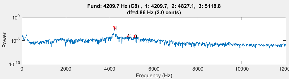
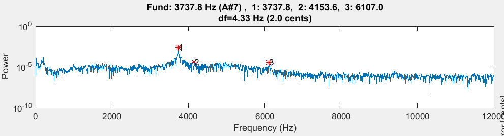
Notice that the peak is not well defined. By contrast, here are the PSDs for bars 42 and 44:
Bar 44 PSDBar 42 PSD
These two have much more well defined peaks than bar 43. We looked back at the PSDs for the blanks, and the differences were not as obvious, so we couldn’t have caught this before tuning. We considered remaking this bar but ultimately decided it was good enough. Perhaps we will replace it in the future.
Here is what the bars sounded like at this point:
All sound pretty good except for the B7 bar, which, as noted, sounds a bit dead.
Just for fun, here is a sped-up video of me tuning on of the bars:
As you can see, I move back and forth a lot between the sanding and tuning stations.
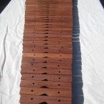
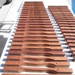
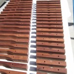
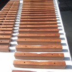
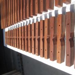
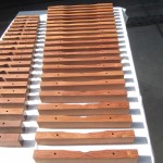
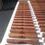
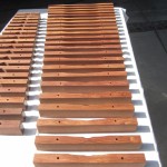
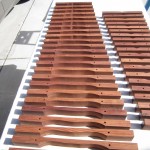
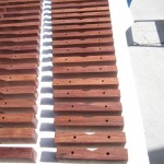
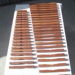
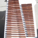
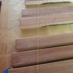
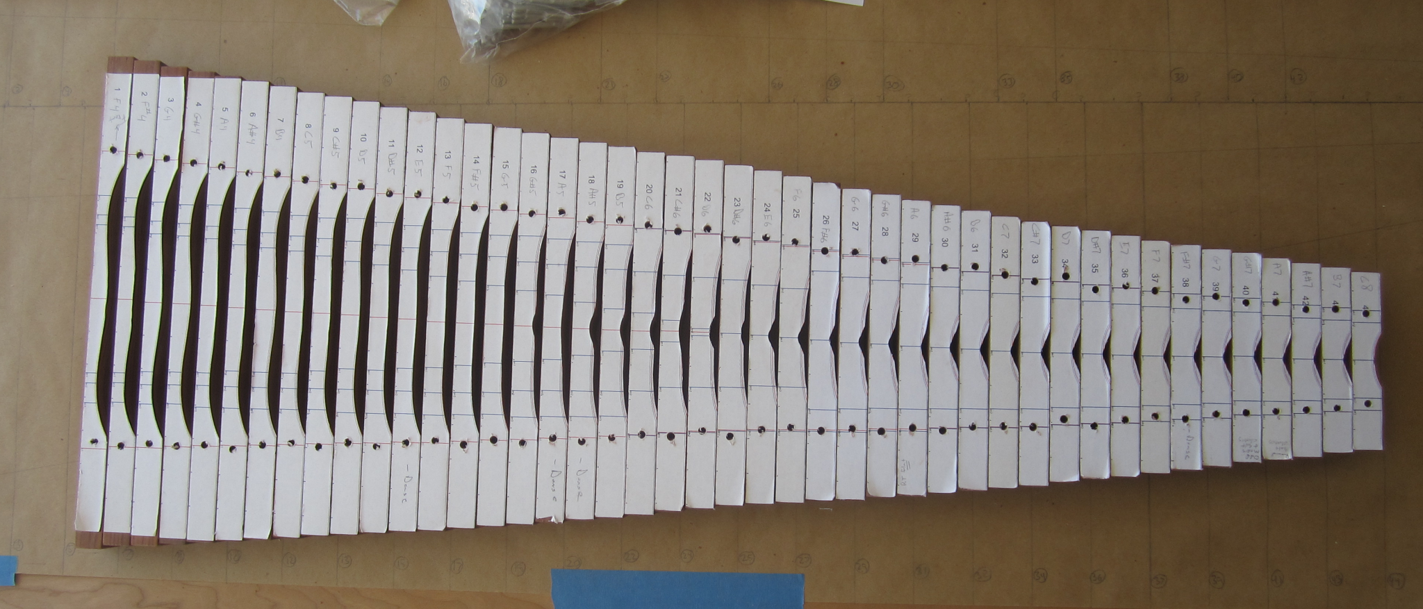
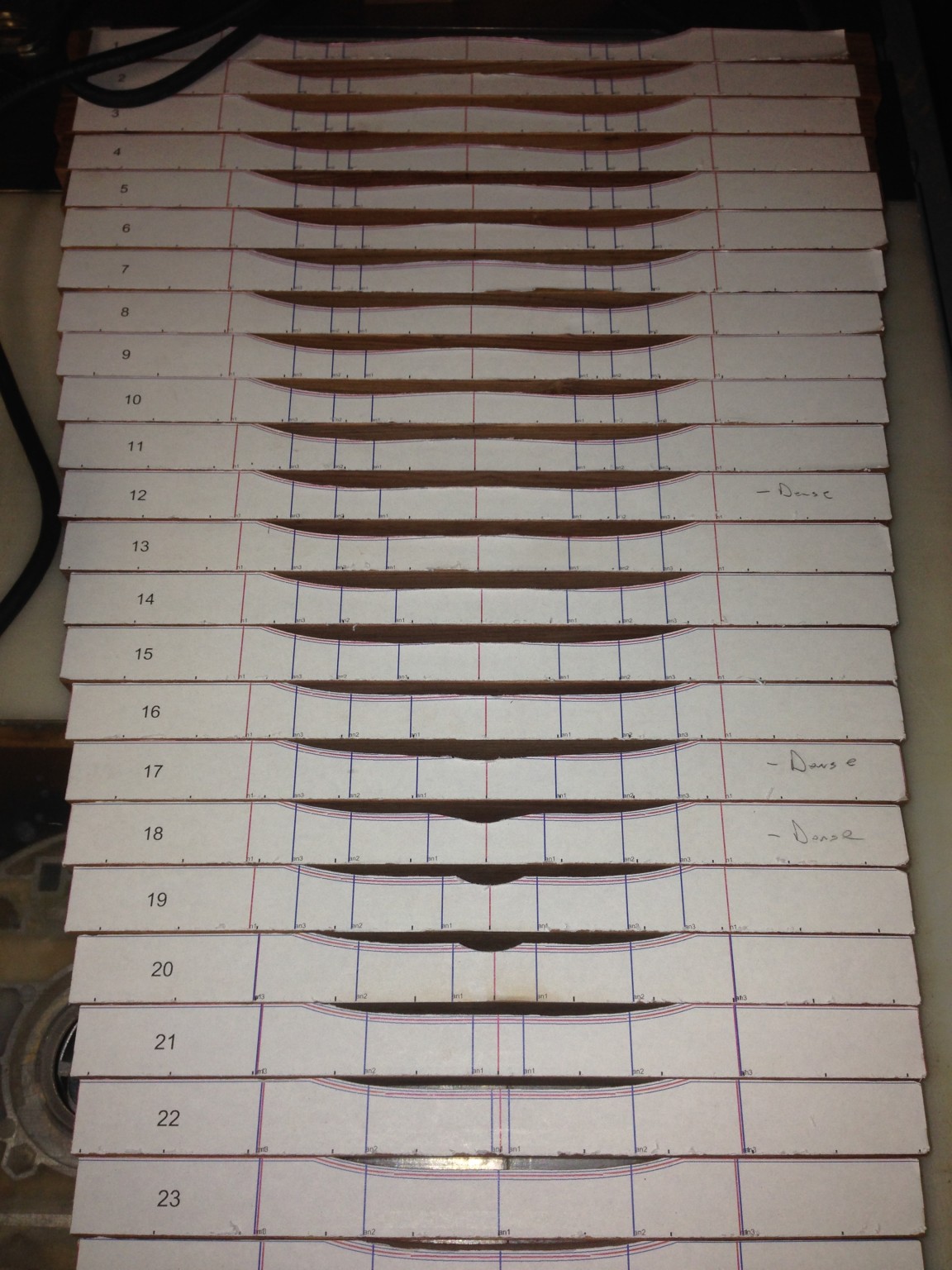
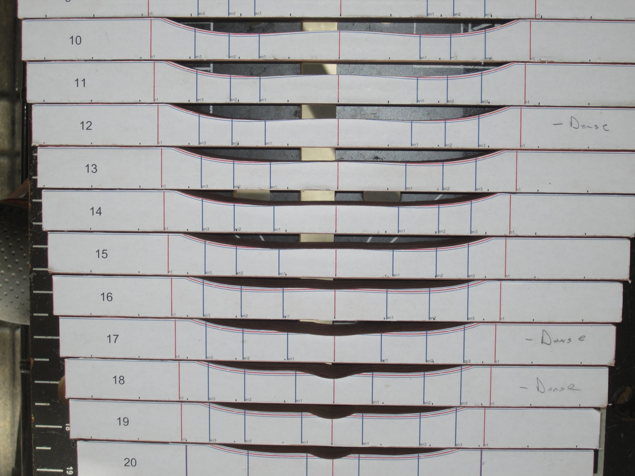
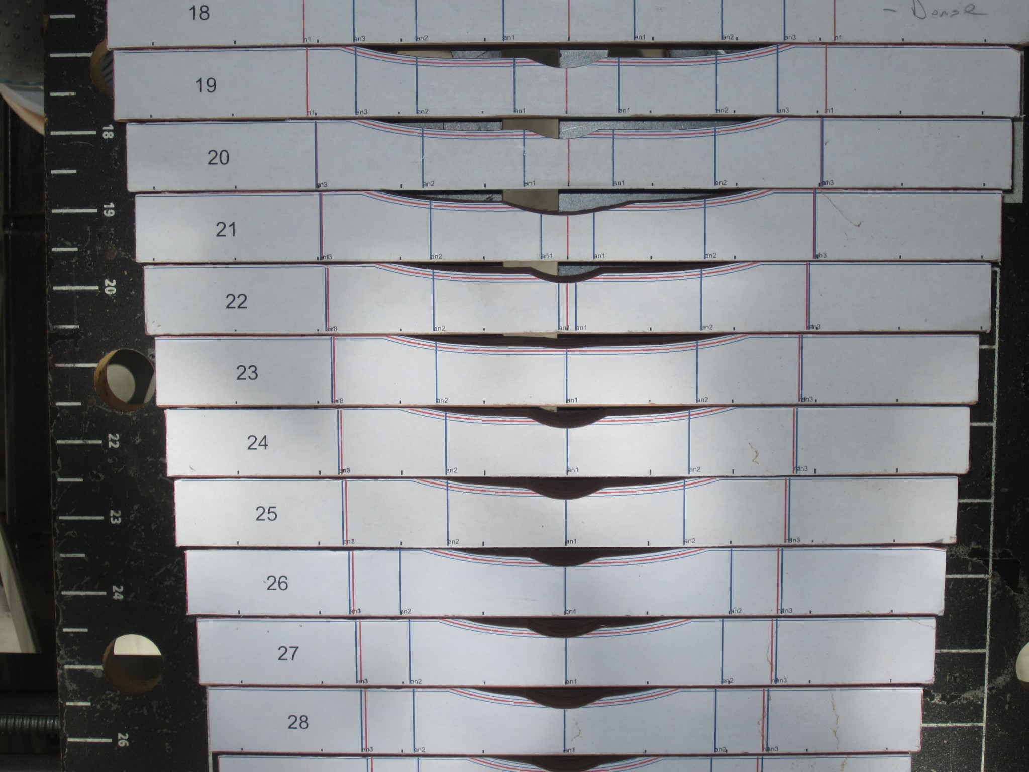
After tuning, I removed the labels and cleaned them up a bit. Here are a bunch of pictures of the bars:
Invoice for resonator tube material
Our tuned bars
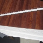
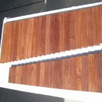
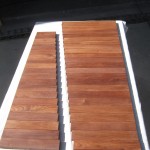
Too many photos of our tuned bars (hey, we were proud of work!)
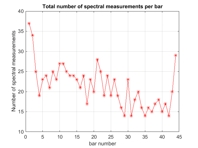
Finally, if you are thinking about building your own bars, you might be interested in the following plot, which shows the number of times I made spectral measurements of each bar.
Number of spectral measurements per bar
This included all of the initial measurements (i.e., of the blanks) and the rough and fine tuning. This also include a tweak or two that we performed after the fine tuning. As you can see, my longest and shortest bars took the most sand/measure iterations, since I was still learning. After I had these tuned, I worked my way from longest to shortest (i.e., bar #2 to bar #43). Once I got good, the long bars took about 20-25 cycles and the short bars were somewhat faster. All told, this was 939 total spectral measurements – a lot of time and patience.
How Long Did All of This Take?
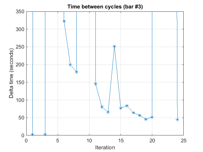
You may be wondering how much time each sand/measure cycle took (I did,) so I plotted the time between spectral measurements for a typical bar.
Time between sand/measure iterations for bar #3
At the start, the when I was removing more wood, the cycles took perhaps 5 minutes. However, as I got closer to the final target frequencies, I was removing just a bit of wood, so the tuning approached 1 minute per iteration.
For round numbers, let’s assume each iteration took, on average, 2.5 minutes. The total time for bar tuning, then, is 939*2.5 / 60 ~= 39 hours. That’s a lot of tuning time! If I had to do this again, it might be a bit faster; at the end of the day, however, I don’t know that there is any way to speed up these cycles without the risk of overshooting the target frequency.
With the tuning essentially done, Jack and I moved on to building the frame and fabricating the resonator tubes. Stay tuned to hear more about that…
The last lengthily post described the method and results for the rough tuning of our 44 bars and described a few challenges that we encountered along the way. Here we are going to describe the process of determining the suspension hole locations and the actual drilling.
To simplify construction of the xylophone, it would be best to have the cord that suspends the bars follow a straight line; this allows straight support rails and straightforward placement of the suspension posts. Also, all of the commercial instruments that we inspected were built with straight suspension cords.
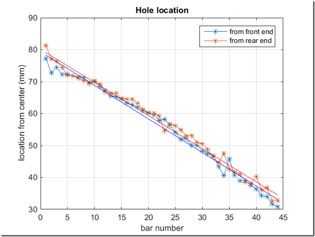
Having measured all of the node locations using the salt method, we were able to assess how linear the node locations were and how much they would deviate from a straight line. The next plot shows these results.
Hole locations with linear trend lines
The symbols are the measured node locations from the front and rear ends of each bar (we define “front” to be the bar ends that face the player). There is clearly a gentle deviation from linear, but it is modest, so I chose to ignore it. Doing otherwise would force me to mount the suspension posts along a curve, which would obviously complicate construction.
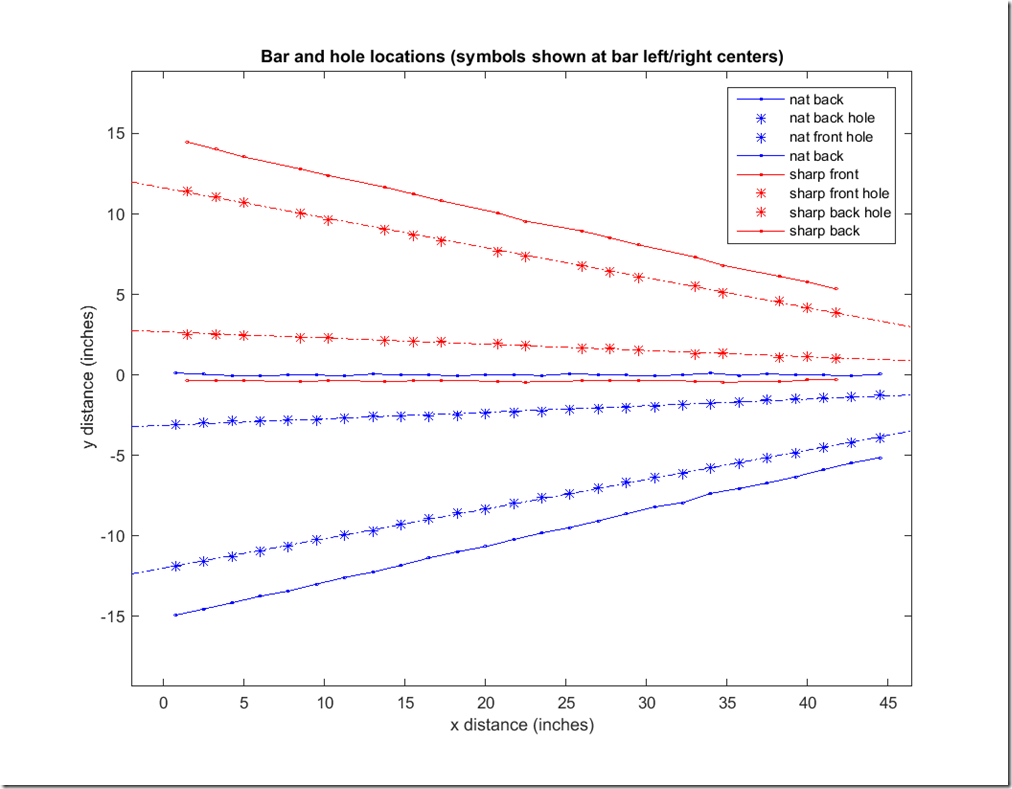
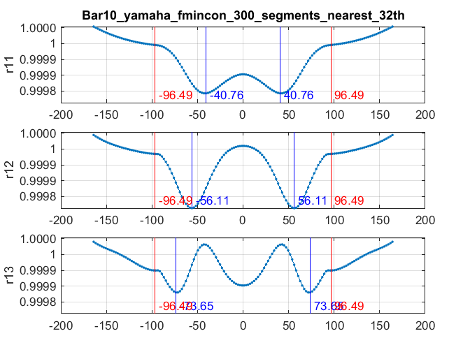
Of course, the holes must be drilled at an angle relative to the bars. To figure out the hole angles, I wrote a little code to plot the locations (as if you were looking down on the instrument). I left 1/4 inch spacing between the bars, which might be a little tight for mounting posts, but I can space them a bit more later if needed (this, of course, affects the angle slightly, but the change is negligible). The following figure shows the output of this code.
Bar and hole locations
There is a lot going in this figure, so let me explain. The plot basically shows the location of the bars’ ends and posts in physical space. The blue solid lines show the locations of the natural bar ends. The red lines give the same info, but for the sharp bars (also called the accidentals). As you can see, the front edge of the sharp bars overlaps the back end of the natural bars. This is allowed, as the rear bars are elevated. In general, it is desirable to have the accidental bars as far forward as possible to minimize the reach needed by the player. The asterisks show the measured node locations for each bar, and the dashed line is the best linear fit through the node locations. If you look carefully, you will note that the solid lines (the bar end locations) are a bit wiggly. This is because I shifted each bar for and aft (actually Matlab did it) to split the difference between the best-fit line and the node locations. I did this to minimize the distance between the linear fit and the true node locations. Aesthetically, this is somewhat undesirable (i.e., the bars ends are not perfectly lined up,) but results in more bar sustain, since the damping due to the mounting string is minimized.
The hole angles that I computed from Matlab were
Natural front hole angle (deg): 10.4
Natural back hole angle (deg): 2.3
Sharp front hole angle (deg): -2.2
Sharp back hole angle (deg): -10.5
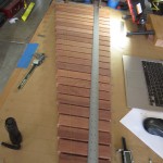
Jack and I started marking all of the computed node offsets on each bar, but this got pretty tedious. In the end, we laid them out carefully on a piece of craft paper that had markings for the horizontal locations and then empirically adjusted the bars to get the best fit to a straight line. Here are a bunch of photos showing the layout and alignment to the penciled node locations:
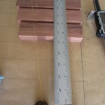
The yellow thread was stretched between two posts to establish a perfectly straight line. As noted above, we visually scooted each bar to try to minimize the distance between the yellow thread and the penciled node marks. When we got them sufficiently aligned, we laid down a 4 foot straightedge aligned with the thread and marked the compromise hole locations on each bar.
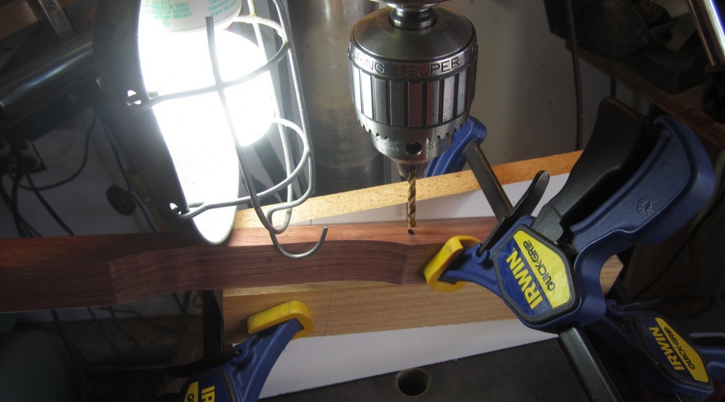
Finally, at the top of the page is a picture of the drilling operation. We faced a 90 degree cast iron angle block with a piece of 3/4 inch melamine that had lines for the 2.2 deg and 10.5 deg marks drawn on it. We clamped on a stop block aligned with the marks to keep the bar from sliding down the melamine as the holes were drilled. For the 10.5 degree holes, we used a center drill to start the holes to avoid bit wander and then finished the holes with a 3/16 inch drill bit. Here is a photo of all of the bars with the drilled holes:
All bars with drilled holes
The red lines near the holes of each bar correspond to the computed node locations. The agreement is between these computed locations and the drilled hole locations is generally quite good.
In the next post, we will move forward with the fine tuning after which we will have almost completely finished bars!
In the last post, Jack and I turned all of our blanks into shaped bars by cutting and sanding a bit proud of the computer-generated profile line. Now we had to “rough tune” them in preparation for drilling the suspension holes. I had previously noted that drilling the holes had almost no effect on the frequencies for our maple test bar. However, I did a quick test on a much shorter bar and found a significant “flattening” of the fundamental mode. We decided to rough tune each of the bars to about 50 cents sharp to pre-compensate for the hole drilling.
Temperature and Humidity
In our correspondence, Dr Entwistle and I speculated about the affect of temperature and moister content on the sonic properties of the bars. Rodney suggested that perhaps friction heating resulting from the drum sander might affect the spectral measurement. This was a good point, so I decided to do a quick temperature sensitivity experiment.
First, I took one of my prismatic Rosewood bars and measured the spectral characteristics at room temperature to establish a baseline. The fundamental was at 1868.0 Hz at a thermal equilibrium temperature of 18.1 C. I let it soak in the fridge overnight, and measured the cold temperature at 1.0 C. I then removed the bar from the fridge and quickly measured the fundamental to be 1884.8 Hz. I was surprised that the frequency didn’t change more. This is only about a 0.9% change (15 cents) for a 17 deg decrease or about 1 cent/deg. This result was good news, because it suggested that I did not have to worry too much about bar heating during the tuning process.
Moisture content was a different story. The process of developing the tuning process, and the mechanics of tuning 44 bars took months. I purchased the Rosewood in January of 2015, and finished the tuning in October – about 10 months. During this period, I noticed a consistent pattern; whenever I left weeks or months between spectral measurements, I would notice a significant sharpening of the bar frequencies. I suspected that this was due to wood dry-out over time. You may recall me noting that the vendor who provided the wood stated that he had recently received the shipment of Honduras Rosewood – it had not been in Albuquerque long prior to my purchase. I can only speculate where the wood came from, but it is likely that it was from a climate that was more humid than the arid desert of Albuquerque. New Mexico has a typical relative humidity that is typically 10 or 20%, so we are more dry than just about anywhere.
When I first got my Rosewood in January, I measured the density of a couple of prismatic test bars. To establish the density, I weighed the bars and accurately measured the dimensions. This yielded the following densities.
January 2015
rho1 = 1081.7 kg/m^3
rho2 = 1082.1 kg/m^3
Just today I re-weighed the bars and re-calculated the densities as
February 2016
rho1 = 1042.4 kg/m^3
rho2 = 1041.9 kg/m^3
This is about a 4% decrease in density over 13 months. Wow! This will certainly have an affect on the bar frequencies.
I guess the lesson is that one should properly season the wood to their local climate prior to tuning these bars. (Anectodally, Dr Entwistle suggested letting the bars acclimate for a year or so prior to shaping them, but I was just too eager to get to cutting!) In any case, I lucked out in that the bars got sharper, rather than flatter over time. Recall that it is much easier to decrease the modal frequencies than it is to increase them. This would have been a serious mistake if I lived in a more humid climate, such as Florida. This is another big “lesson learned” for those of you out there who may be attempting to build your own instruments.
Back to Tuning…
First, we re-cut the three bars that were sonic outliers. This was not a big deal, but did involve all of the familiar steps (ripping, planing, jointing, sanding, etc.). It’s so much faster the first time when you are doing it in volume! We also printed new labels and got them adhered to the bars. The frequency response on these new “blanks” was in family with the bars around them, so we were comfortable moving forward with shaping.
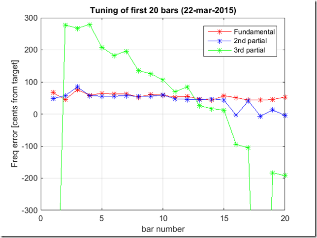
In our first run at tuning, we got 20 done. We were shooting for about 50 cents sharp on both the fundamental and first partial. The graph below shows the current state of our first 20 bars.
Modes for the first 20 rough-tuned bars
As you can see, the first and second partials are well behaved for most of the bars. The third partial, which we decided not to tune, wanders around similarly to other xylophones that we had spectrally measured.
Note that as the bars got shorter, the computer-generated bar shape became less accurate. As you can see on bar 16, 18 and 20, the second partial is tuned about perfectly (not 50 cents sharp, as targeted). This is not due to my tuning, but rather because the second partials for these bars were already closely tuned directly after band-sawing the shapes ~2 mm proud of the computed profile. To tune these bars, I removed wood only at the center of the bar to minimize the affect on the second partial. As you can see in the following photo, these bars shapes have deviated quite a bit from the computer prediction.
First 20 rough-tuned bars
Over the subsequent weekend, Jack and I were able to get the rest of the bars tuned. Here are the tuning results:
Frequency characteristic of all rough-tuned bars
The fundamental on all bars was pretty good except for bar 29 (my A6 bar,) on which I must have daydreamed while sanding, thus making it a bit flat. I thought that I might need to fix that bar, but that turned not to be the case since the moisture dry-out sufficiently sharpened the bar prior to fine tuning. The second partials above bar 21 (C6) were mostly flat even with the +2 mm rough sawing. However, I was not concerned, because this is consistent with other xylophones that I measured. For example, here is the tuning for the Kori xylophone that I measured:
Measured spectral tuning graph for Kori xylophone
As you can see, for the bars above C6 the second partials for this xylophone are whacky or too quiet to measure.
The photos show that, starting at bar 18, I had to cut a very narrow notch at the center to yield the desired tuning. As noted above, this is because the rough-sawed shape already had a second partial that was close to the +50 cents desired. As I’ve said previously, the computer predictions start to break down for the shorter bars (as a point of reference, bar #18 is about 11.5 inches long). I don’t think that this is due to inconsistency with a single bar, because the issue seems systematic for all of the “shorter” bars.
Another limitation that I found with the computer results concerns the tuning curves. For example, here is the tuning curve for bar 21:
Tuning curve for bar #21
This curve shows a subtle sharping of the 2nd partial for wood removed at the center. The trend gets more pronounced for the shorter bars. However, I saw no evidence of this when removing wood at the center. I typically saw no change in the second partial with wood removed from the center. As I’ve discussed previously, all of this is likely just a limitation in the approach (i.e., bar theory).
An Improvement?
Later, after doing all of the rough tuning, it occurred to me that I could have modestly improved on my approach to the computer predictions. Specifically, since I performed frequency measurements for each of the Rosewood blanks, I could have used these to compute the modulus for each bar. I could have used this, plus the measured densities for each bar to compute the bar shape for each bar’s paper template. (Recall that I used a single average modulus value and density for all bars.) While I am guessing that this would have reduced variability between the predicted and measured bars, I doubt that it would have significantly improved the systematic issues I saw with the short bars which are most likely the result of the “plate-like” geometry of the shorter bars. Nevertheless, using the per-bar modulus and density seems like a better approach and one that I would recommend.
Wrapping Up the Rough Tuning
Because the computer predictions only approximate the nodal locations for bar, Jack and I used the “salt method” to determine the actual node locations. Here are a few photos. First, is a photo of the salt results for a long bar, including the pencil marks I drew through the salt “mounds.”
Salt test results for a typical long bar
Here is one of the shorter bars, before and after strikes with the mallet:
Salt sprinkled on short bar (prior to mallet strikes)Salt test results (after mallet strikes causing salt to migrate)
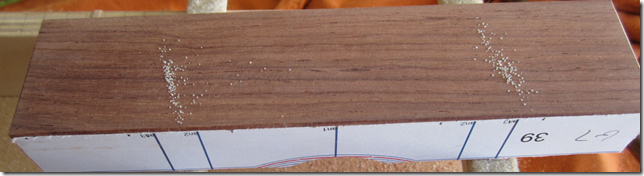
The salt results for bar #40 were curious – the nodes did not form lines at all, but rather fairly circular clusters as shown here:
Salt results for bar #40
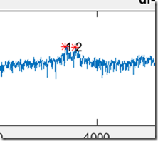
This one also had an atypical spectrum, as shown here:
Unusual spectrum measured for bar #40Zoom of bar #40 spectrum
The zoomed plot shows that there were two modes that were very close together. Compare this to bar #39, which was typical of the spectrum for most of the short bars.
Zoomed spectrum for bar #39 showing typical results
Bar #39 shows a nice, single discrete fundamental mode.
Dr Entwistle suggested that perhaps the two close modes that were were observing with bar #40 was the result of a torsional mode closely coinciding with a bending mode. We spent a bit of time trying to ring up the torsional modes to test this theory, but found it difficult. The La Favre site showed some torsional mode results, but that was for marimba bars which are substantially wider.
Bar #40 definitely seemed like an outlier. It also sounded a little different than the others – perhaps a little less “bright” than its neighbors. Jack and I considered remaking this bar, but in the end, decided that it wasn’t worth the effort, given the subtle effect.
The Sound
Here is a sound file containing all of the rough-tuned bars:
A few notes on this sound file:
The mallet double-bounced on some of the strikes, which you can hear.
You can hear a “warbling” for the first few bars. This is due to the Doppler effect that result from the bar bouncing on the rubber-bands of the tuning jig after the bar is struck. As an aside, this warble is perhaps a few Hz so I later wondered if it could be broadening my spectral peaks and reducing the accuracy of my spectral measurements. A modification of the tuning jig that utilized e.g., felt strips rather than rubber bands would have addressed this potential issue.
You may also be able to hear the flat A6 bar.
Having rough-tuned all of the bars, I guess if I were going to do this again I might do some sanity checks along the way to identify anomalous bars early to avoid unnecessary work. For example, after cutting each bar to length, but prior to sanding, attaching the label, or rough-cutting the under-shape, I would probably do a quick spectral check and do the salt method. Then, I could reject any bars that were out of family with the rest. For example, I would check for:
A fundamental or second partial out of family with the rest
The double peak in the fundamental (like my bar #40)
Out of family salt results (i.e., weird nodes)
This quick up-front work could save some considerable re-work down the line.
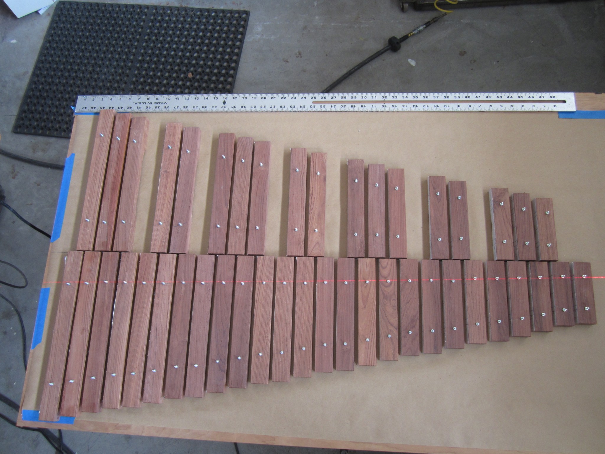
As a teaser, here is a photo of our 44 bars in an approximate lay out. Pretty cool to see it becoming an instrument!
Rough tuned bars laid out in there approximate configuration
Jack and I were ready to go into production for our 44 Rosewood bars. All of the previous discussion about the maple bar is apropos here too, but I will fill in some details of the construction process.
Our First Two Bars
We made two bars first, the longest and the shortest, so that we could ensure that the math and process that we developed for our maple bar also worked for the Rosewood.
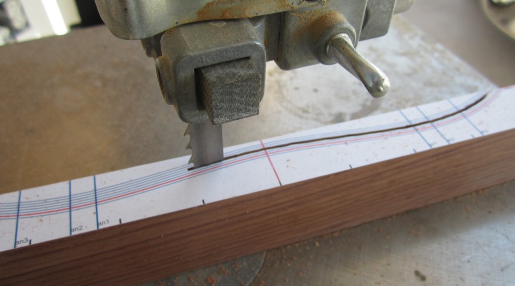
One part of the process that I didn’t show for the maple bar was adhering the paper template to the bar. It is pretty important that this be aligned accurately with the wood, so I developed a technique that used my daughter’s light table. This photo shows the configuration that I used.
Paper template and alignment block on the light table
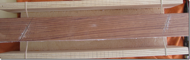
The picture shows the light table with a piece of window glass on top to extend the flat surface of the table (since the longest bars were longer than the light table), and a large block of wood that we used to align the bar with the template. We sprayed the bar side with 3M adhesive to attach the template. If you’ve ever used this stuff, you know that you only get one chance to align the two pieces – there are no do-overs. So we would put the paper template on the glass face down and then carefully align the wood block to the top edge of the bar profile printed on the paper. We penciled a small center mark on the bar that allowed us to ensure that we had good left/right centering. Then, with adhesive on the bar edge, we would carefully slide the bar down the alignment block, while taking care to align the center marks on the bar and the template. Here is a photo of the bar correctly aligned to the template:
Bar aligned on template
There is not much to see in this photo, because the bar completely covers the printed lines on the paper. Paper was stuck to the bar, we would use a sharp razor to trip the paper flush with the bar. Here is a photo that Jack took of me trimming the template:
Trimming the template
Blanks and Templates
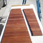
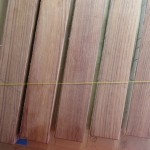
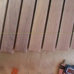
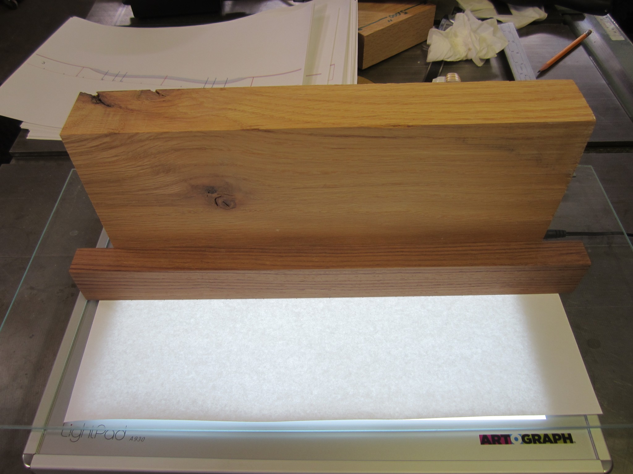
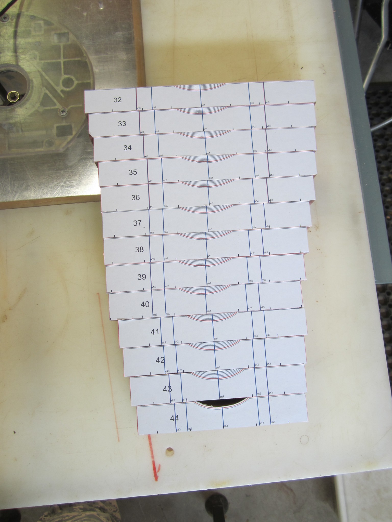
To say the least, attaching all of the paper templates is a bit tedious, but works well. Here are a couple of photos of the 42 “blank” bars with the templates attached (2 were already shaped as described below).
Long blanks with templatesShort blanks with templates
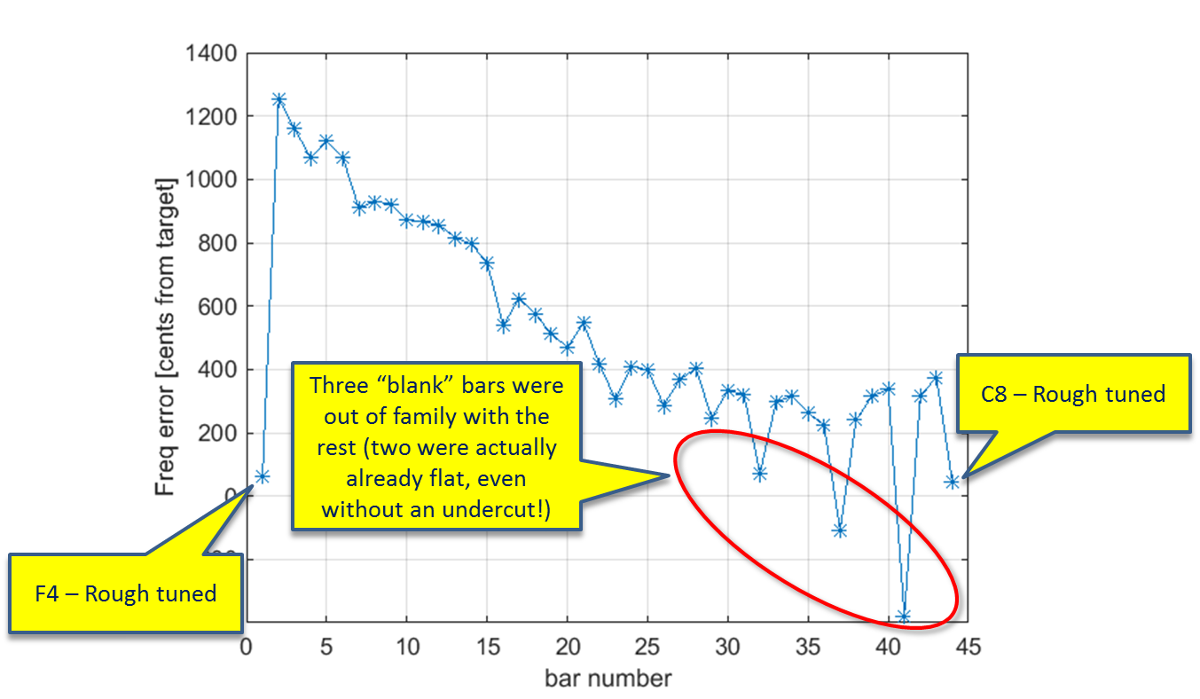
After attaching the templates, the first thing I did was spectrally measure each of the bars to establish a baseline. This is when I discovered that three of the bars were spectral outliers. The following figure details this finding:
Plot showing spectral outliers
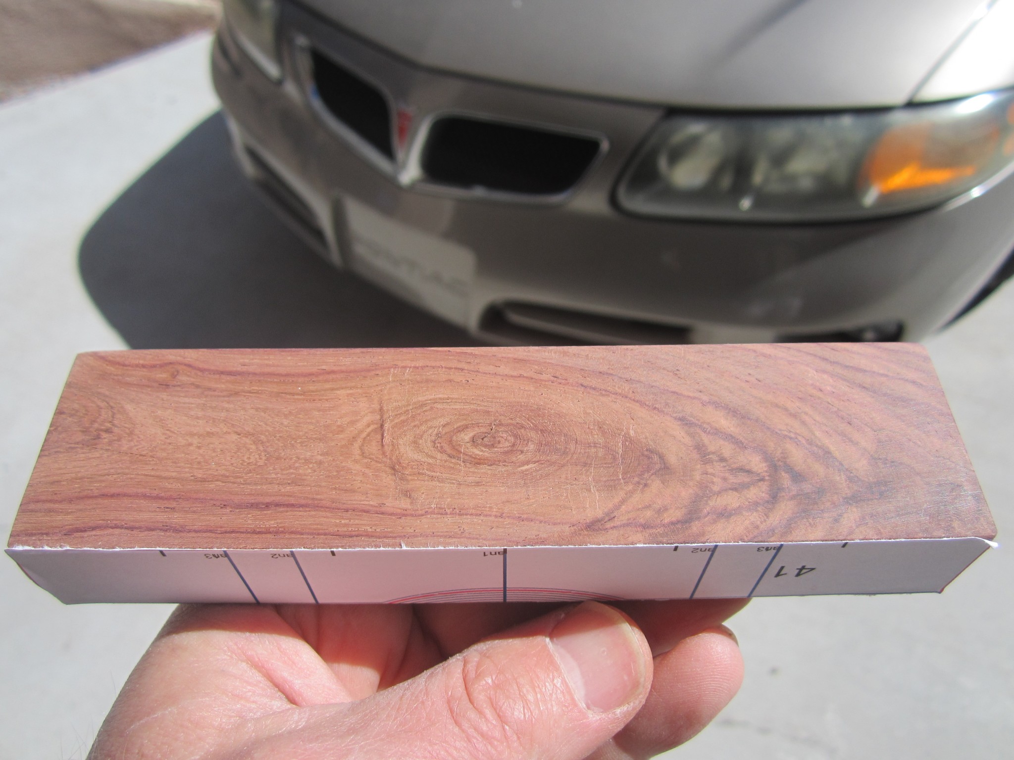
This figure plots the error in the fundamental mode (quantified in cents, relative to the desired target frequency). The first and last points corresponded to my F4 and C8 bars which we had previously “rough tuned.” The three bars inscribed by the ellipse are the outliers. Notice that these are “out of family” relative to the rest. Two of the three were actually already flat (relative to the target frequency). For one of the bars (#41) I anticipated there might be a problem, as it had a knot in the center. Here is a picture of that bar:
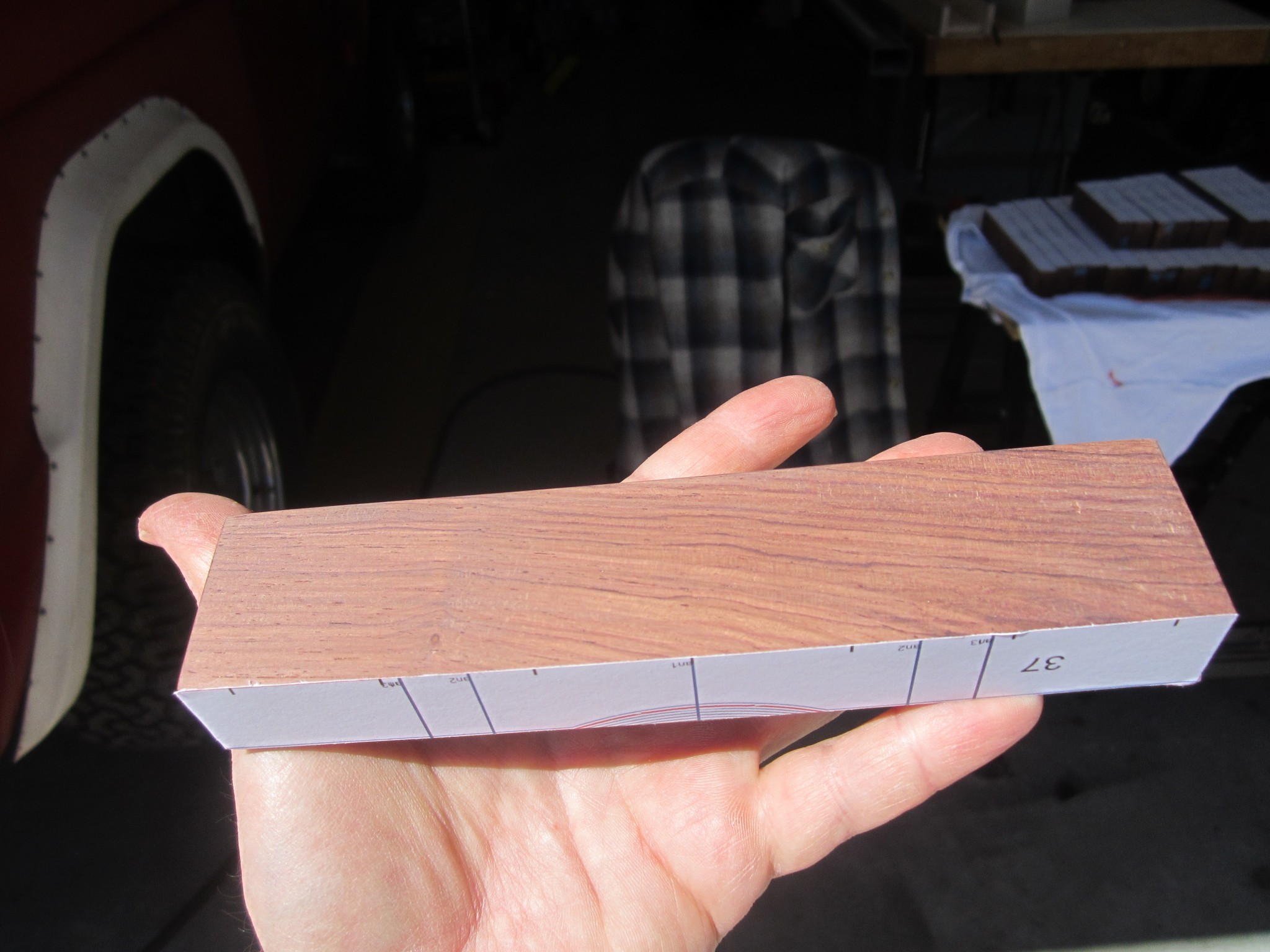
Bar 41 with the knot in the center
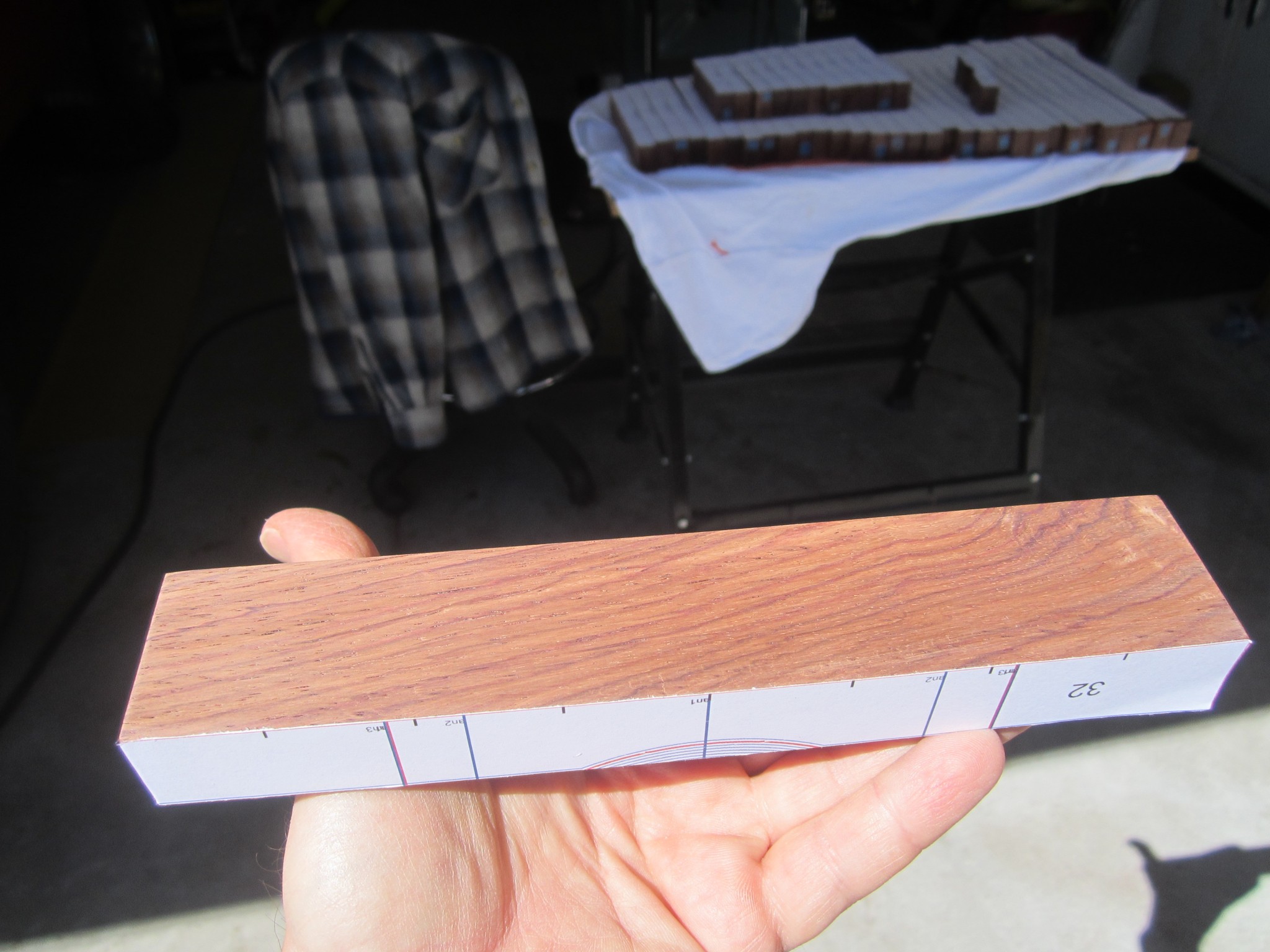
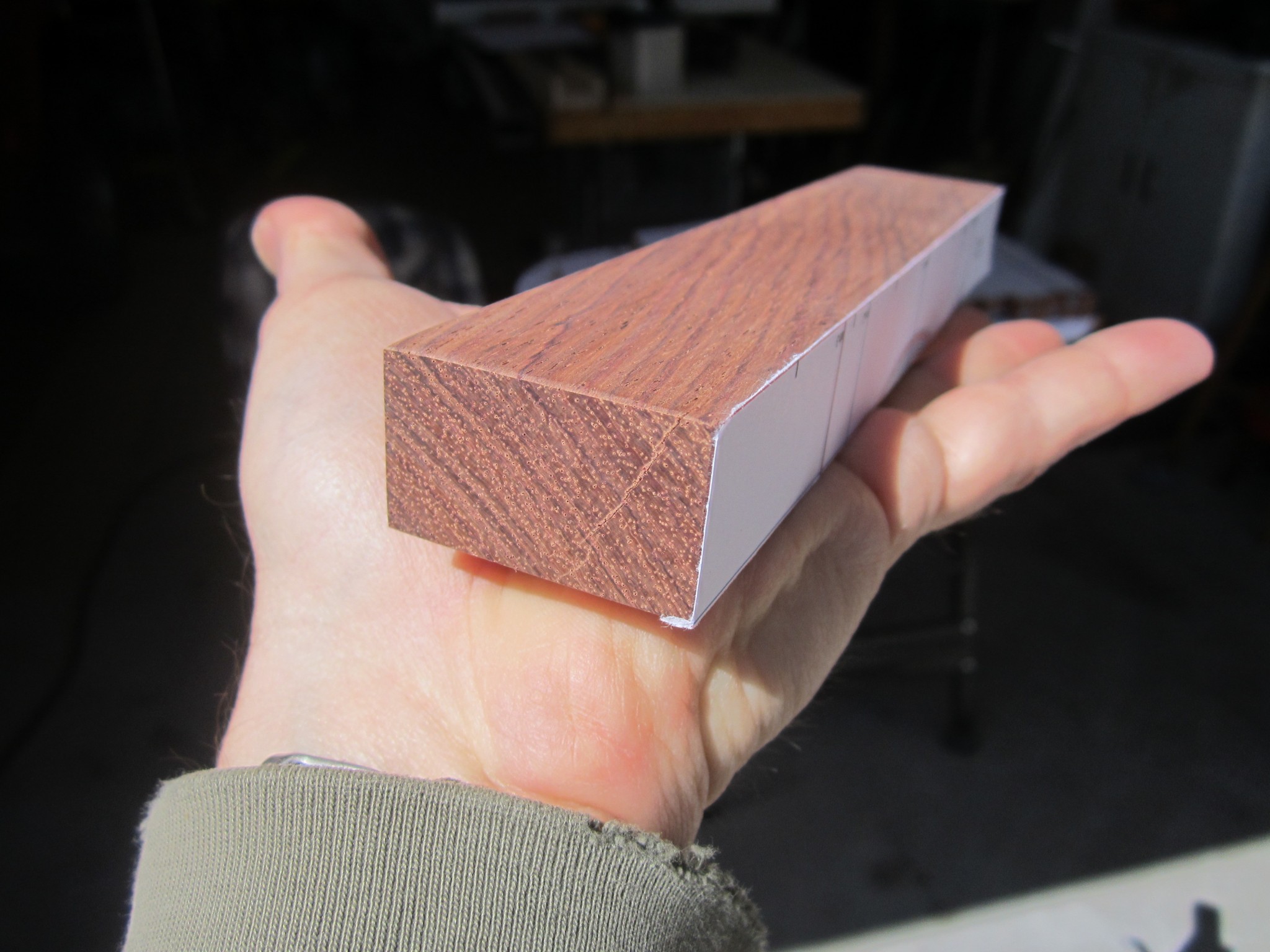
Of the other two, one had some slight checking in the end which may have been indicative of a more systematic issue with that chunk of wood. I could find no issue at all with the third bar. Perhaps it had some internal flaw. Here are some photos of those two bars:
Bar #32Bar #32 showing checking at endBar #37 – No apparent reason for flat mode
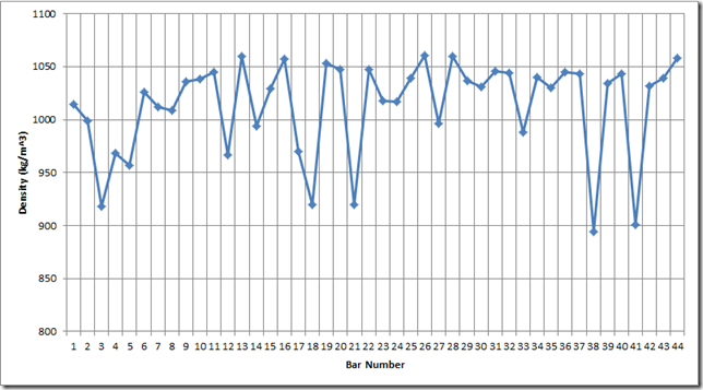
In order to determine if perhaps the unusual sonic results for these three bars might be related to density, I weighted each bar and computed the density. The tabulated density values are in the Excel file included in the previous post and are plotted here.
Density of bar blanks
While the density of bar 41 looks way low, the densities for the other two anomalous bars look “in family” with the rest of the measurements. Further, there are other bars, like 18 and 21 that have low densities but in-family sonic characteristics; so it does not appear that the unusual behavior is related to density variation. As a side note, I wish that I had kept track of which bars came from which boards; I suspect that the bars with low densities all came from the same board.
I ended up making three new bars to replace these funky bars. Luckily, I purchased some extra rosewood – throughout my woodworking forays, I have learned that I consistently underestimate the amount of waste that results during construction and have gotten better at compensating.
In any case, there was a fundamental lesson in this finding: to save effort, it would be wise to do a spectral analysis of each bar just after dimensioning the blanks in order to identify outliers. In my case, I wasted a bit of time sanding the bar surface smooth and attaching the labels prior to measuring the frequencies.
Shaping the Wood
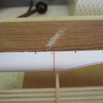
At the top of this post is a photo of the first band saw cut for our rosewood F4 bar – the longest bar.
Like the maple bar, I sanded a bit proud of the computer generated red bar profile line. Here is a photo of us sanding the bar:
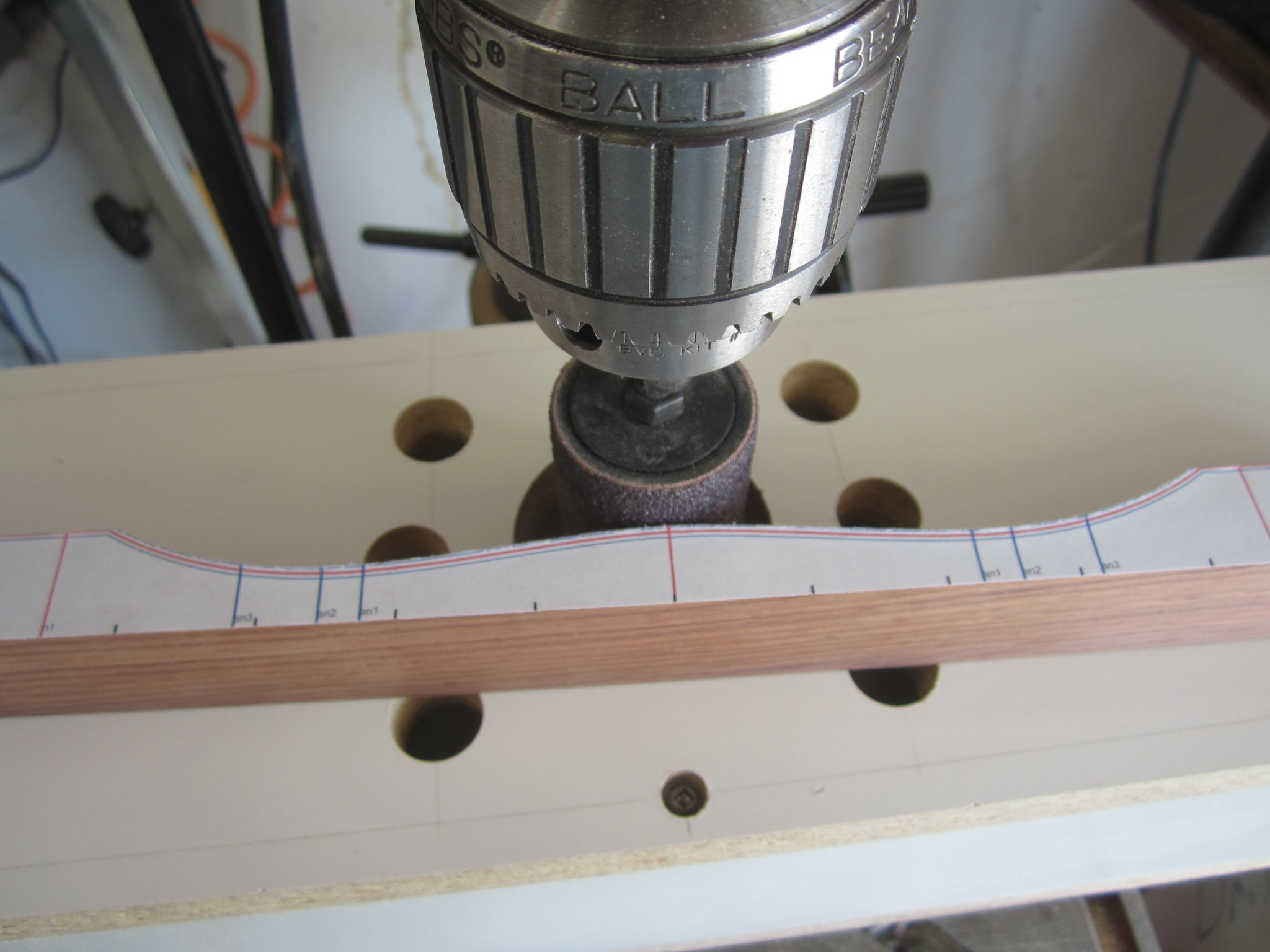
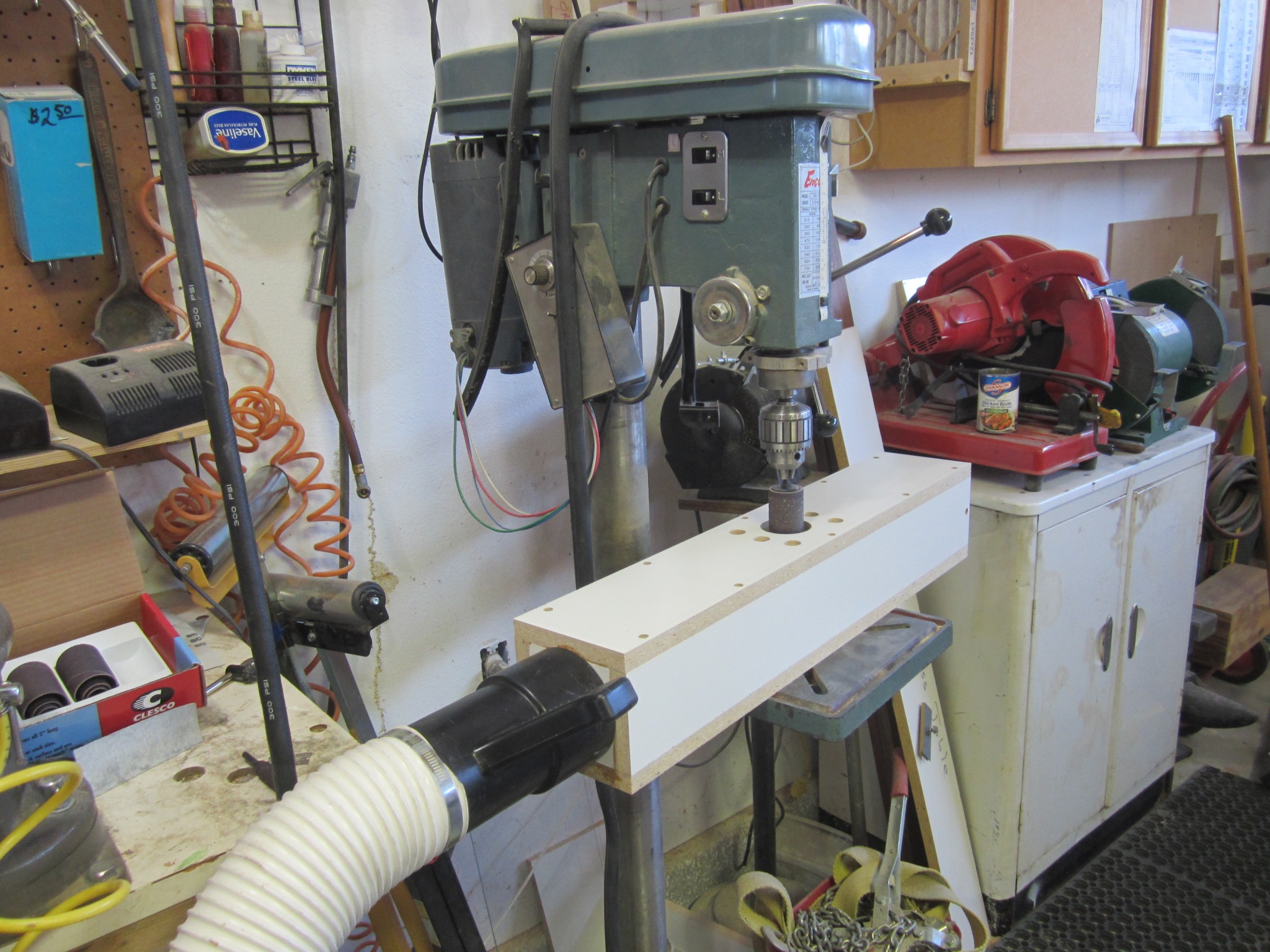
Sanding the F4 bar
This is just a 2 inch drum on my drill press. The white base with the holes is a melamine box that I built to collect dust. This sanding produces a lot of rosewood dust which can cause allergic reactions in some people, so I wanted to capture as much of it as I could. Also, sucking the dust away as we sanded allowed us to more easily see the paper template lines. Here is a full picture of the box:
The sanding rig
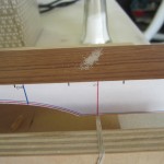
I left the bar about 50 cents sharp, which was a fraction of a millimeter above the computer prediction line. Out of curiosity, I did the “salt test” on this bar to see verify the node locations. Here is a picture:
Randomly scatter salt prior to the salt migration
Migrated salt
Zoom of left end
Zoom of right end
You can see that the salt locations match very well with the predictions from the code – super cool!
We cut and tuned the shortest bar, which is a C8, by sanding to about 1 mm proud of the shape line predicted by the Timoshenko code. In this case, I was only about 36 cents sharp. In general, the assumptions underlying the beam theory break down for these shorter bars, so the computer predictions get worse. Dr Entwistle pointed me to a good paper by Oyadiji that described the use of 3-D Finite Element (FE) modeling and “plate theory” (as opposed to “beam theory”) to predict the modal behavior. However, as I have stated, I was not too concerned about tuning the overtones for the higher bars since they are negligibly affect the timbre. I just needed the code to predict shapes that got me in the ballpark since the final tuning is iterative anyway.
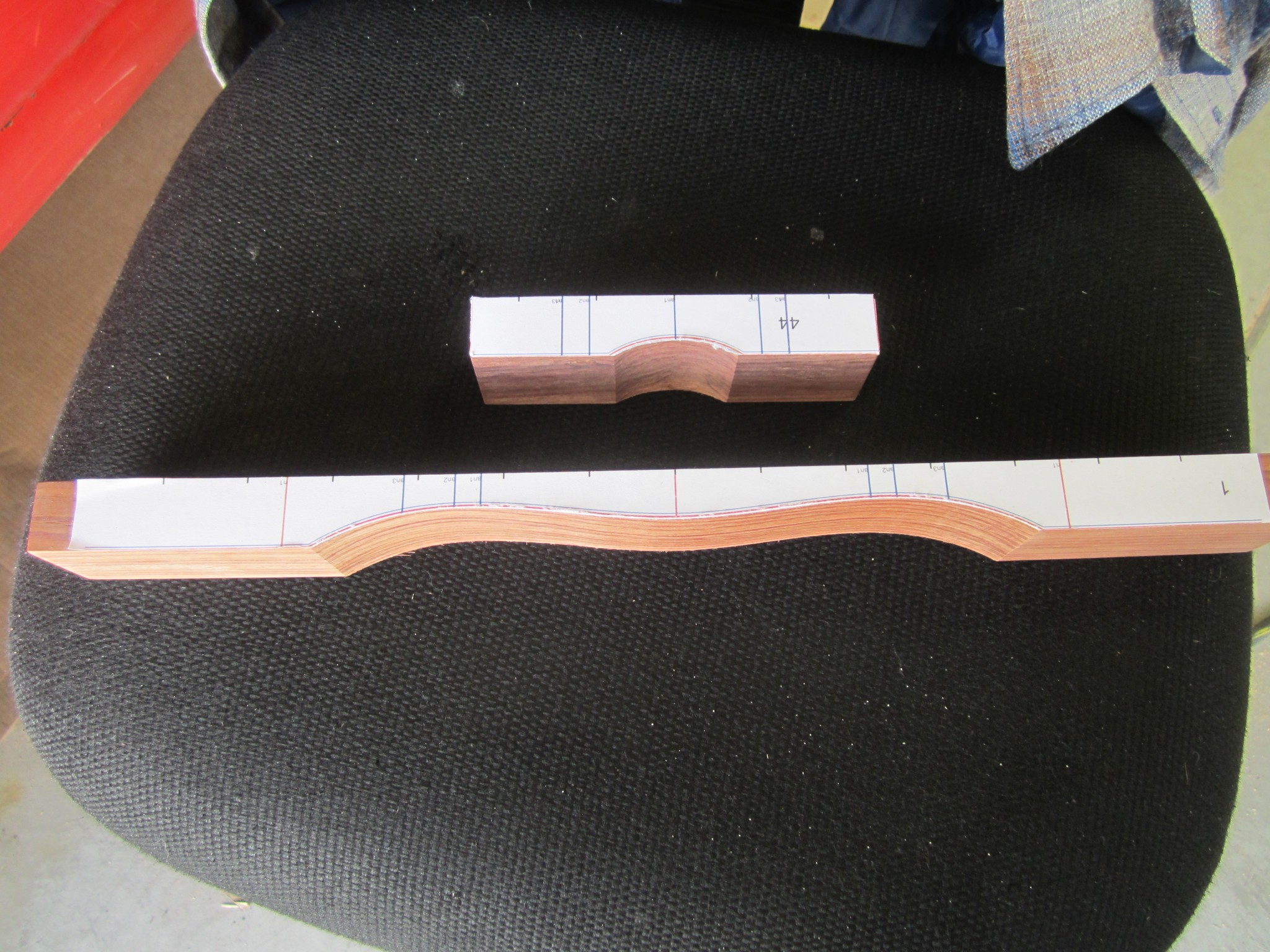
Here is a photo of my longest and shortest bars with the templates attached and the rough shaping complete:
Our longest and shortest bars
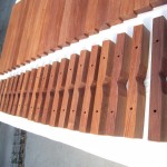
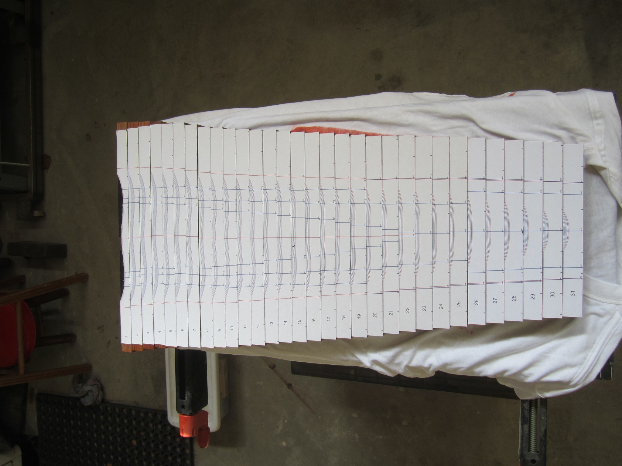
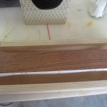
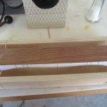
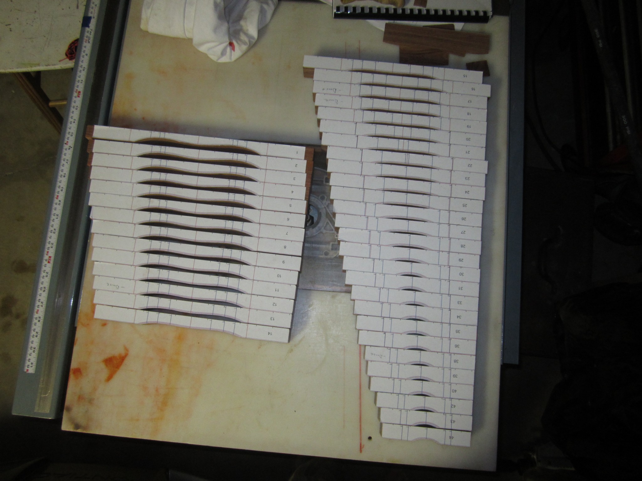
Having had success with cutting and measuring the two bars, we set out to fabricate the other 42. We started by roughly cutting the shape on the band saw. This went much faster than I anticipated and only took a couple of hours. I spent another couple of hours on the drum sander with two goals: 1) remove the saw marks 2) sand to a constant distance from the red computer-generated profile. I wasn’t trying to get all bars to have same standoff distance from the red profile but rather, for each bar, I was just trying to maintain a uniform distance from the red profile. This meant that some bars were 1 mm proud of the red profile, and some were 2+ mm proud. In any case, here is a photo of our 41 “good” bars (i.e., we hadn’t remade the three wacky bars yet).
Bars after sawing and rough sanding
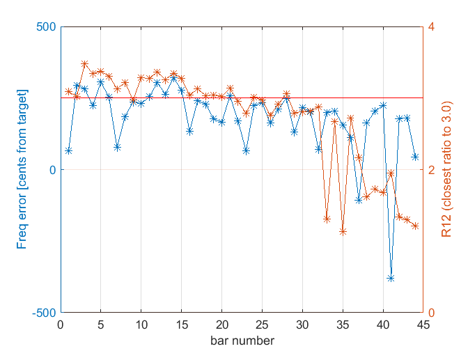
Now, the critical step was to spectrally measure each of the bars again to ensure that I had sufficient frequency margin to drill the holes and do the final tuning. As I established on the maple bar, the holes had a nearly negligible effect on the long bars, but holes I drilled on a short blank (a remnant that was shorter than even my C8 bar) demonstrated a +2% change in frequency. Here is the result this second spectral analysis:
Spectral results after rough sawing and uniform sanding
As you can see, all of the 41 “good” bars have a fundamental frequency that is higher than the target; this is great! Plotted in red is the ratio of the first overtone (relative to the target frequency). Note that the code to compute this really just searches for the ratio that is closest to 3.0. Consequently, if the first overtone doesn’t have enough energy to measure, then the code will just find the fundamental, which happens typically happens for bar 32 and above.
As we’ve discussed, I really only care about the second partial on the first 25 or so bars. Beyond that, I doubt that the second partial has enough energy to be audible. Surprisingly, a few of the bars already had a R12 ratio that is < 3.0. This means that I removed a bit too much wood on these bars. During the tuning process, I tried to address this issue, but you will hear more about that later.
Finally, for fun, I will leave you with a wave file that contains the an audio measurement for each bar. Note that the frequencies are not monotonically increasing at this point, since they are just the frequencies that resulted after doing sanding to the uniform offset from the profile. In any case, it is kind of cool to hear the actual bars.
References
S Olutunde Oyadiji and Raad Ali, “Finite element modal analysis of free-free beams and plates: A study of transition from beam-like to plate-like behaviour,” Twelfth international congress on sound and vibration July 2005
In the previous posts, I described the basic construction and tuning of a maple xylophone bar and promised that we would get into the woodworking next. However, we’ve got to do a bit more math first. Sorry for another bait-n-switch….
Rosewood Properties
As you may recall, the computer code that computes the bar shape requires the bulk modulus, shear modulus, and density to be specified. Apparently I am incapable of learning a lesson and again turned to the internet to provide these numbers. Like many of my previous attempts, I came up empty handed. Considering that all great Xylophones and Marimbas are made of one material – Honduras Rosewood – you might think that someone would have posted the material properties on the internet. If they did, Google and I couldn’t find it. This left me determined to compute them myself.
I did find a range of values for Young’s modulus (aka the bulk modulus) in a paper by Brémaud, et al. Figure 3a of the paper provided Young’s modulus values for Honduras Rosewood (latin name Dalbergia Stevensonii) that span the range of 17-26 GPa. I am not sure why the range varied so much. Perhaps it is just natural variation in the wood? As an interesting aside, figure 3b of that same paper clearly shows that Honduras Rosewood has the lowest damping coefficient of all of the species evaluated, which the paper suggests is perhaps the most important quality for wood used to construct idiophones- this wood really is special.
But the Zhao paper (and a few others that I found) came to the rescue. Appendix B of that paper, “Calculations for the Mechanical Properties,” provided a formula for calculating Young’s modulus from the fundamental frequency of a prismatic beam constructed from the material. My first job was to whack a Rosewood bar of known dimension and measure its fundamental. I had a couple of rosewood “test bars” that I cut to mess around with, and the longest one was 13-5/64 inches long. Here is the spectrum of that bar.
Spectrum of my longest rosewood test bar
And here is the sound file for your listening pleasure.
From the spectrum, you can see that the fundamental was at about 957 Hz. You can check out the Zhao paper for the details of the equation, but here is the Matlab code to compute the modulus. (Note that the Zhao paper had an error in equation for E where beta_n should have been the constant beta_n*l)
inch2m=0.0254; %Conversion constant

%Compute the young's modulus from bar #1
b=1.501*inch2m; %width
h=0.880*inch2m; %height
L=(13+15/64)*inch2m; %Length

f1=957; %Measured frequency of fundamental
rho = 1082; %Density from measurement of volume and mass (see above)

A=b*h; %Cross sectional area
I=b*h^3/12; %Moment of inertial

E=4*pi^2*rho*A*L^4/I * (f1^2/4.73^4) %4.73 is a constant given by Zhao
%E = 2.396974370897572e+10
The modulus calculated for this bar was 23.9 GPa. I had a second bar that had a length of 9-27/64 inches and a fundamental frequency of 1867 Hz. The calculated modulus for this bar was 23.6 GPa – pretty close to the first number.
Zhao also gave a formula for the calculation of the shear modulus, G, but the torsional frequencies of the bar must be known. It was not clear to me that I could adequately “ring these up” and measure them, so getting the shear modulus using that approach seemed off the table. I decided to take a different tact.
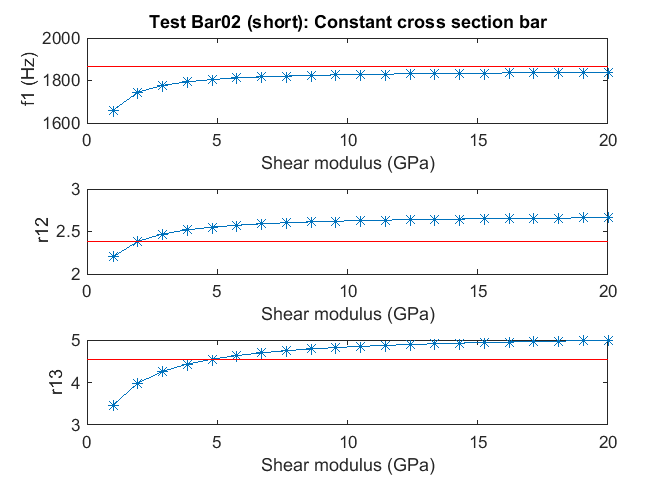
My approach was to do a parametric sweep of the shear modulus using the Timoshenko code to compute the fundamental and first two overtones for a prismatic beam. My idea was that if I had the bulk modulus and density right (density was easy, I just weighed and measured the bar and divided the numbers,) then the only free variable was shear modulus. If I adjusted it until I made the Timoshenko-predicted frequencies match the measured frequencies, then I must have the right value for the shear modulus; right? Here are the results from that sweep for the long and short test bars.
Shear modulus sweep for my long test bar.Shear modulus sweep for my short test bar
The red lines on the plots correspond to the measure modal frequencies based on my spectral measurements. This analysis was not entirely satisfying because the no value of G yielded the fundamental frequency – the prediction was always a bit lower than the measured value- however, inspection of the second and third partials suggested that a reasonable value for the shear modulus might be around 4 GPa.
For what it’s worth, I did find a published shear modulus value of 19 GPa for Padauk, a similar wood. This suggests my chosen value of 4 GPa might be too low, but I wasn’t sure what else to do – high values resulted in a very poor match for the overtones in the plots above. For what it’s worth, I computed some bar profiles with different values of G, and they didn’t vary a lot. So perhaps at the end of the day it’s not a big deal, since I knew I was going to have to “hand tune” the bars after roughly cutting to the computed shape anyway. Right or wrong, I forged on with my value of G=4 GPa.
Summary of Computed Results
With the Rosewood material properties estimated, I was able to run the minimizer/Timoshenko code to compute the bar profiles for each of my 44 rosewood bars. As I mentioned in a previous post, the minimizer is sensitive to the initial starting condition, so I seeded my first and longest bar, F4, with the cubic coefficients from the maple bar and watched the minimizer converge. For the rest of the bars, I initialized the minimizer by seeding it with the coefficients from the previous bar, working my way from longest to shortest. In this manor, I was able to leap-frog through the bars and ensure that the minimizer converged.
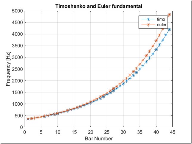
Here are some summary results from the computed bar runs. First, here are the fundamental frequencies as calculated by the Timoshenko and Euler methods for each of the bars.
Computed fundamental frequency for all bars via two different methods
In every case, the code was able to perfectly converge to the desired fundamental frequency. The plot shows the results for the two methods. As previously noted, the Timoshenko method is generally more accurate, especially for the short bars.
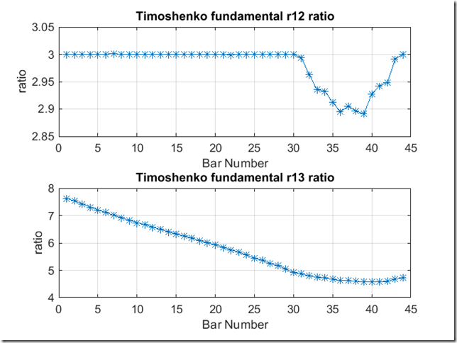
Here are the ratios for the second and third overtones:
Computed ratios for the first two overtones
I found it interesting that the code can’t converge on the 2nd overtone for the short bars. No big deal because the overtones decay so rapidly for the shorter bars, it is doubtful that this effect can be heard. Indeed, when I was tuning the shorter bars, my spectral measurements were not able to measure the overtones.
The Templates Please
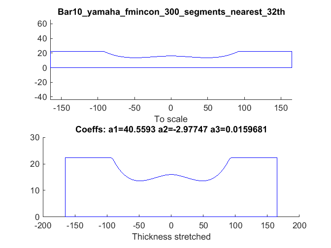
The computer run for each bar produces three standard plots. The first is the bar profile plot. An example for bar 10 is shown here.
Profile plot for bar #10
You’ve see plots like this before. The top figure has a 1:1 aspect ratio and gives an idea of the actual physical profile of the bar. The bottom figure has a arbitrary aspect ratio to better visualize the shape of the undercut. Also included on the figure are the coefficients for the cubic function that describes the profile curve. I followed Dr Entwistle’s definition for the cubic coefficients where
y=a1*x^3 + a2*x^2 + a3;
In this equation, x is the longitudinal length down the bar where x=0 is the bar center. The variable y denotes the bar thickness corresponding to each value of x. Notice that when x=0, the equation reduces to y=a3, which is the thickness at the center. Also, notice that there is no linear term with x (i.e., no coefficient that multiples x). Setting the linear coefficient to zero forces the cubic function to have zero a slope at x=0. This forces symmetry about the bar middle.
Note that there is nothing magical about using a cubic to represent the bar shape. Indeed, if I were going to build another xylophone, I might mess around with other functional forms to see if I could satisfy additional constraints, like forcing the third partial ratio to be 6.0, or to maximize sustain or volume. However, the cubic is a good compromise in that does a respectable job of providing shapes that mimic what I had seen on other xylophones while keeping the degrees of freedom low (i.e., just 3 coefficients).
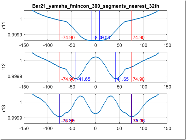
The second standard plot that I compute is the tuning curve, which we have discussed at length. For completeness, here is the tuning curve for my #10 bar.
Tuning curve for bar #10
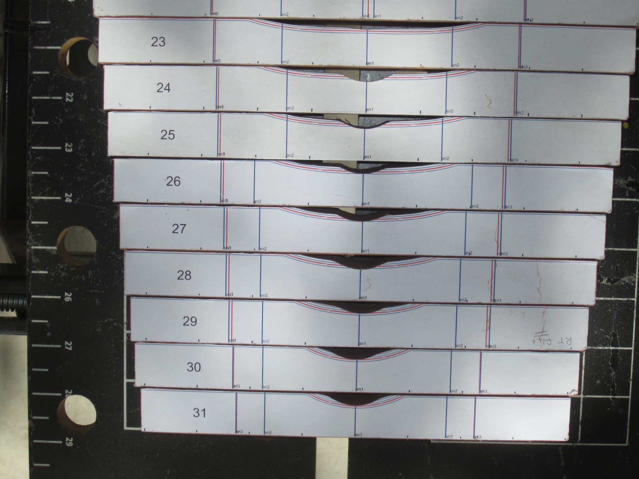
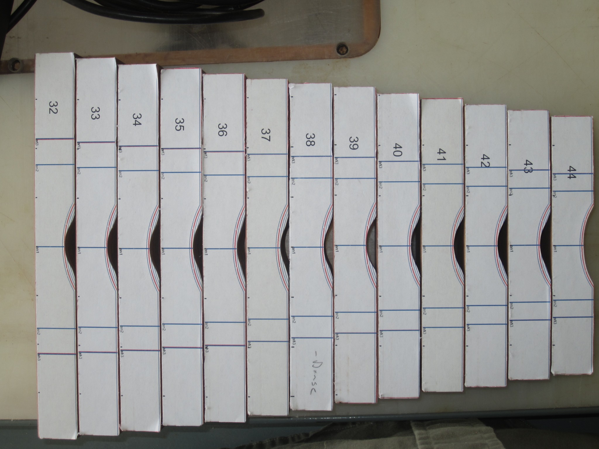
Finally, as described in the maple bar fabrication discussion, I create a full-size paper template for each bar. Here is the template for bar #10:
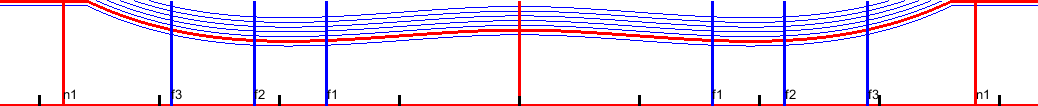
Template for bar #10
A couple of notes about the annotations on this template are in order. The two vertical red lines mark the node locations as computed by the Euler code provided by Dr Entwistle. These are where the holes will be drilled. The vertical blue lines, marked f1, f2 and f3 denote fiducials on the bar corresponding to the tuning curve peaks. The f1 mark denotes the location where the fundamental is most affected by wood removal. Similarly, f2 marks the location where wood removal most dramatically changes the second partial, and f3 corresponds to the most sensitive region for the third partial.
All of these are useful plots, so I have zipped up the three curves for each of the 44 bars into a single file for you to download…I am just that kind of a guy 🙂
Note that each of the files is a PDF, including the bar templates. The templates’ PDF files have been created so that they should print full-size. I made these to print on 8.5 x 14 inch paper, which was the largest size that my printer would handle. I am not sure how they will print on a smaller page size, but in any case, you should be able to scale these based on the bar sizes that I provided in the Excel file in the previous post.
In the next post we will actually start cutting Rosewood. (I know, you’ve heard that before. But you didn’t think you could build a xylophone without math, did you?)
References
Iris Brémaud, Pierre Cabrolier, Kazuya Minato, Jean Gérard, Bernard Thibaut. Vibrational properties of tropical woods with historical uses in musical instruments. Joseph Gril.International Conference of COST Action IE0601 Wood Science for the Preservation of Cultural Heritage, Nov 2008, Braga, Portugal. pp.17-23, 2010. <hal-00808403>
With our newfound knowledge of tuning xylophone bars, Jack and I were prepared to go all in – time to buy the rosewood.
We live in Albuquerque, which is not a large city, so I was prepared for a protracted search for affordable rosewood. I found a few sites online, but all were pretty spendy and mostly catered to users buying small quantities. On a whim, I checked out a local vendor called Albuquerque Exotic Hardwoods (now called World of Wood). To my surprise, they had just received a small shipment of Honduras rosewood! The owner explained that there were some “quality issues” so they were selling it for half price.
Like most woodworkers, I typically seek out stock that has the most interesting grain. I generally build furniture that has simple lines and let figure in the wood provide the interest. In selecting stock for this project, I had to fight that urge and select the most boring planks, since these will typically be the most homogeneous. This nearly killed me, and to own the truth, I bought one extra plank that was highly figured and just too pretty to leave at the store.
I know you are going to ask what the price was, and I’ve racked my brain trying to remember, but I’m afraid those brains cells got displaced by bar tuning math. I can tell you that I spent about $200 total on the rosewood. As noted, the wood had some checks and knots that I had to cut around, so I estimate that had about 30% waste. (But did I mention that the wood was half price?!)
The width of the bars doesn’t greatly affect the timbre, so I sized them to be consistent with what I had nominally observed on commercial xylophones. The Yamaha that provided my sizing template had bar width at 1.5 inches, which was right in line with most other xylophones I had seen. The rosewood boards that I bought were mostly about 5-7 inches wide, so for each board I figured out how many widths I could rip out of each plank and started cutting.
When I began ripping these on my table saw, I got my first surprise; despite selecting boards with pretty straight grain, there was so much internal stress in this wood that after ripping the first six inches or so, the piece against the table saw fence (the 1.5 inch strip I was ripping off) started bending badly against the main plank. This is not uncommon when rippling hardwood, but I’ve never seen it this extreme. It is also a serious problem, because as the wood bends out it tends to push laterally against the blade, causing binding and burning. It can also result in pieces that are thinner than the 1.5 inch width target. Not every cut had this problem, but probably half of them did. I am not sure if this is a common problem with rosewood, but I definitely had to address this challenge. So I did two things. First, I ripped the pieces about 1/8 inch wider than the necessary final dimension to allow for thinning that resulted from the bending board.
My second mitigation was to put a screw in the end so the ripped piece couldn’t bend out too far. I wish I had a photo of this, but I didn’t take one, so here is a cheesy illustration that will hopefully make clear how I addressed this issue.
Screw used to capture bending ripping piece
Basically, I would rip the board about 8 inches and them drill a pilot hole at a 45 degree angle. Then, I would drive a wood screw to straighten the 1.5 inch part and pull it back toward the main plank. After this, I would restart the rip, but of course I couldn’t cut through the screw, so rather I would plunge the blade into the existing cut past the screw, then finish the rip cut. This process slowed down the ripping tremendously, but it did tame the board so that I could get decent (not great) cuts. Of course, the resulting ripped boards had a gnarly curve to them, but recall that they only needed to straight over the length of the bar (less than 15 inches).
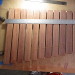
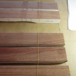
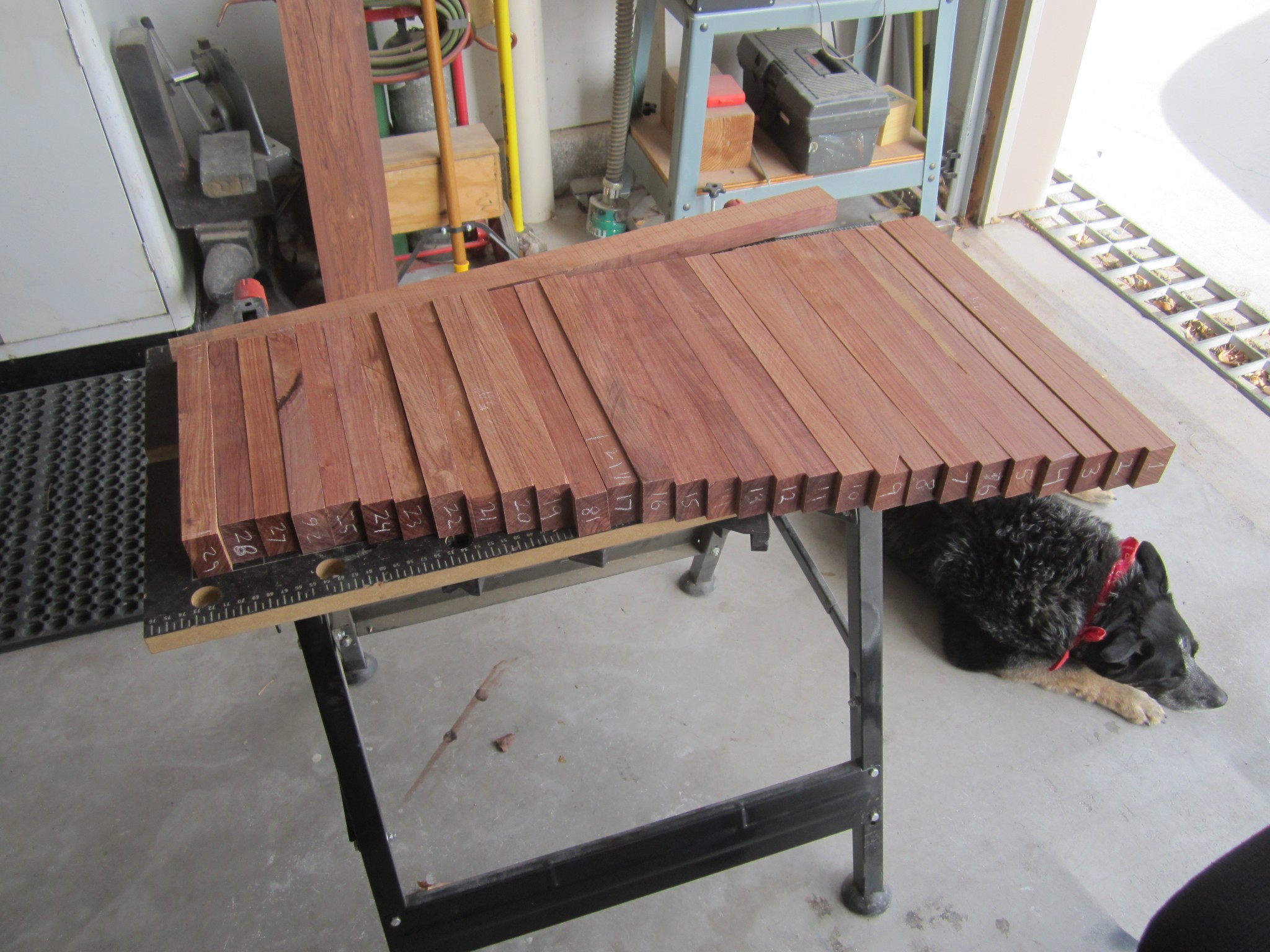
Once I used this technique to rip all of the pieces, I cut out all of the bad chunks. This included knots, splits and checks. This left me with a number of boards that were various lengths, so now I was ready to rough-cut all of my bars from these stock pieces. You can see some of the ripped pieces at the post at the top of this page.
Optimizing Board Usage
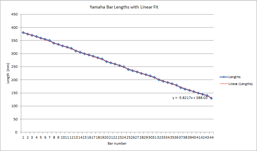
With my boards ripped, the next step was to determine the exact lengths for my 44 bars. Recall from a previous post that I chose to use the lengths from a Yamaha instrument I found online. I entered all of the bar lengths from the Yamaha parts list and created the following plot.
Yamaha bar lengths
There is a bit of wiggle in the points due to rounding in the published Yamaha data, so I added a linear trend line to average out the “noise,” and used that to compute the lengths for each bar. The bar lengths are contained in this Excel file: bar_lengths
At this point, I had my stock ripped to 1.5 inches, and I had exact lengths for each of my 44 bars. Now many times over the years I have ran into the problem of efficiently cutting a number of lineal pieces from a set of stock material lengths. The classic example of this is cutting baseboard molding where you buy nominally 12 foot boards and chop them up according to your wall lengths. In general, the problem can be solved by trial and error – basically guessing at how to best divvy up the needed pieces into the available stock. However, because the rosewood is just a bit more expensive than baseboard molding (pause here to let the point sink in,) I attempted to be as efficient as possible.
I turned back to the internet to see if I could find some software to help. There were a couple of free programs that I found, but they were pretty cheesy and difficult to use. Ultimately, I ended up downloading a trial version of a program called Cutlist Plus. This software is pretty sweet in that it lets you enter all of your stock lengths and the desired finish pieces, and then computes the optimal assignment of pieces to stock. The program takes some getting used to, but it is very flexible and produces very detailed printouts that make it easy to stay organized. I seem to recall that the trial version is good for month. They have a $39 version aimed at hobbyists, but it only cuts sheet goods (i.e., two dimensional pieces like plywood,) not lineal pieces. The full version is $250, which was too rich for my blood. (Please let me know if anyone out there knows of inexpensive software that performs this function – it would be nice to have it around for occasional use).
After rough-cutting all of the pieces according to Cutlist Plus assignments, I dimensioned each bar to it final size. This included straightening on the jointer and ripping to final width on the table saw. Because I cut each bar a bit long, the final step was to cut each to its finished dimension. The Excel file above contains a column with the lengths rounded to the nearest 1/32th of an inch. I find that my table saw rule guide is the most accurate and fastest way to cut short pieces like this, and the fractional column in the spreadsheet allowed me to quickly set the length.
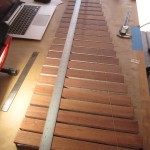
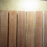
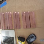
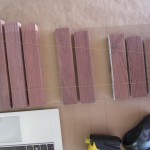
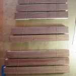
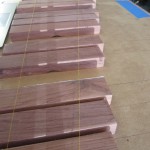
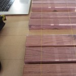
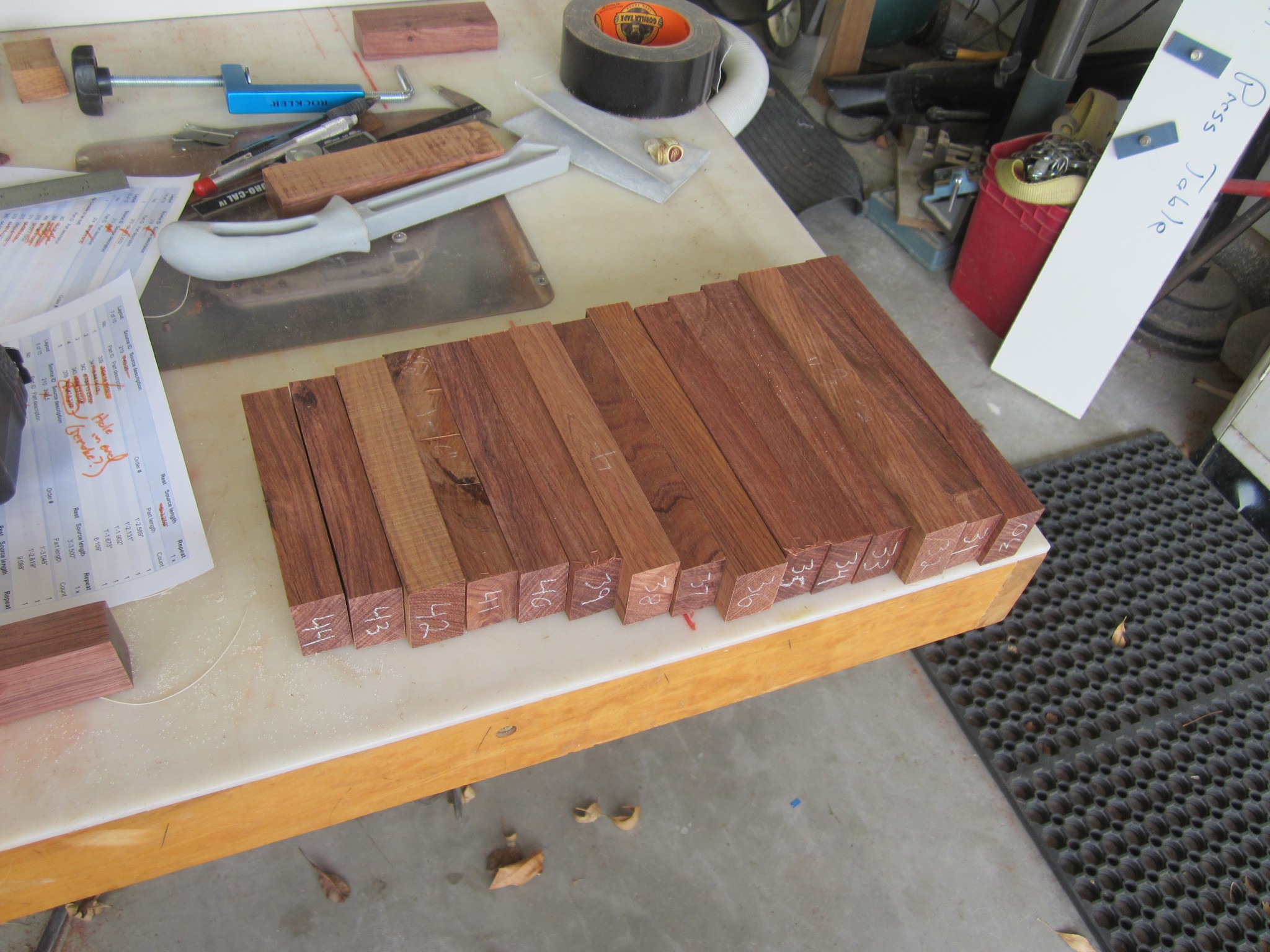
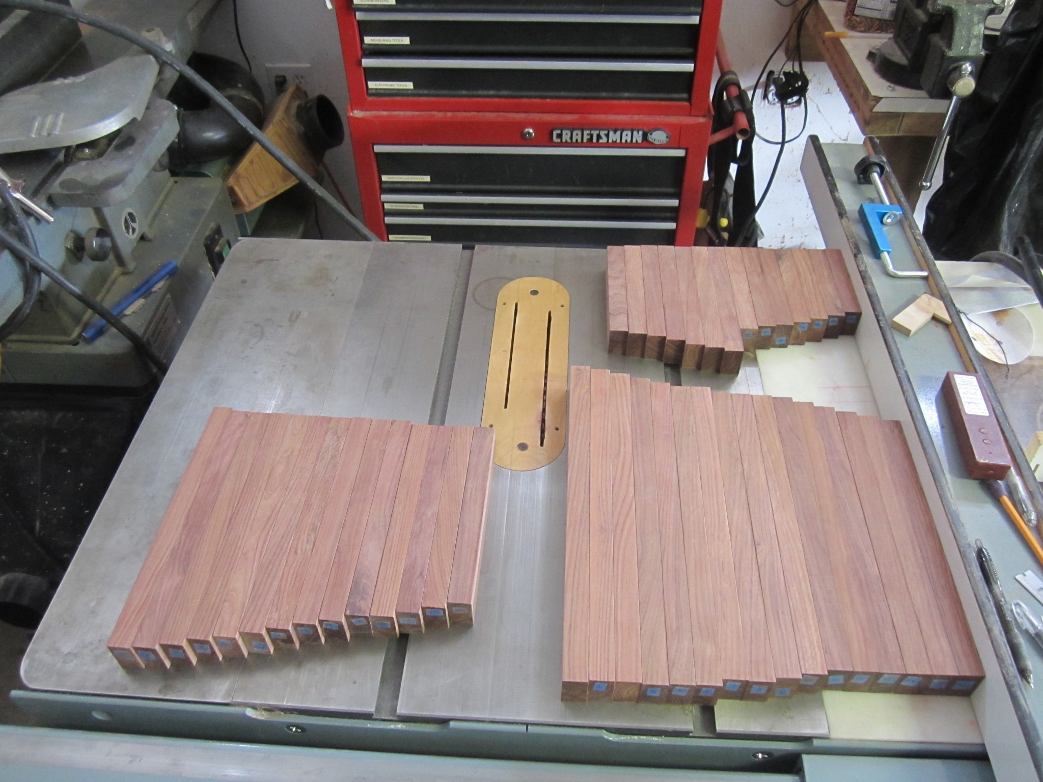
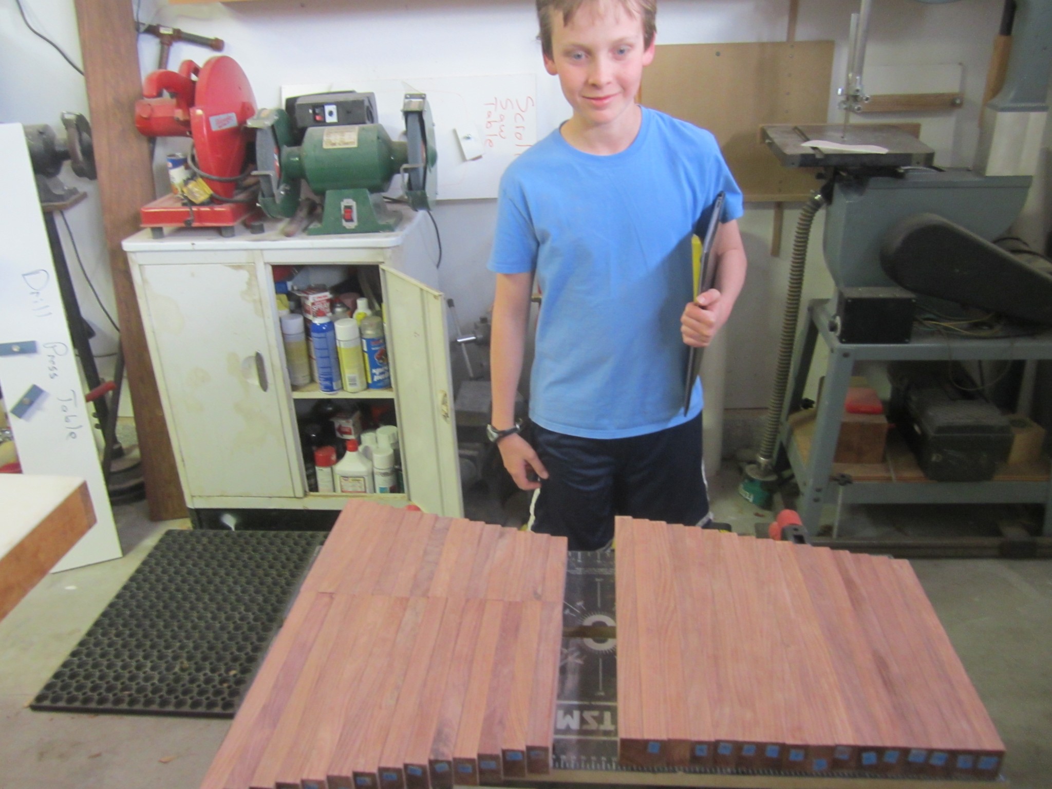
As your reward for staying with us this long, here are some photos of our cut pieces!
Rough-cut piecesRough-cut piecesFinal, dimensioned piecesJack checking out his handiwork!
In the next post, we will show you more of the woodworking steps involved with turning these “blanks” into tuned xylophone bars and a few challenges we encountered along the way.