As noted in the last post, I was only able to find 3 recordings of xylophones on the web that were suitable for spectral analysis. I also described some software that I wrote that spectrally analyzes the clips. In this post, I will discuss some practical implications of the spectral analysis and will discuss some “standard” plots that I use to summarize xylophone sonic performance.

Performance Analysis

We will start with the first sound clip – the c-major scale video example. Below are some plots produced by the Matlab scripts. You will see a lot of these, so I will take a moment to explain each.

Sound Envelope Plot

The plot below shows the sound envelope for the YouTube C major video clip.

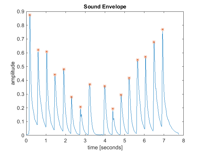
The envelope of the sound clip is basically a curve that contains the amplitude of the sound over time. The example above is typical in that each bar strike produces a sharp peak followed by a decay in the sound amplitude. This information is used to break apart the single sound file into a set of discrete clips that can be individually analyzed. If you count the peaks in this example, you can see that 16 discrete notes were played. This is because the guy played up, and then down the C major scale – he played C, D, E, F, G, A, B, C, C, B, A, G, F, E, D, C.

Spectral Analysis

Once each note is separated out of the sound file, the data can be analyzed to determine the spectral content. A full description of spectral analysis is way beyond the scope of this blog, but there is plenty of information on the web. The basic idea is to analyze the sound bite to determine the power at each frequency. If done carefully, this will show peaks at the resonant modes of the bar. The magnitude of the peak represents the power in each resonant mode, and the location of the peak determines the frequency. By analyzing the series of peaks produced, it is possible to determine how well the bar is tuned.

Well, that is the theory; in practice, it gets a bit more complicated for a few reasons. First, the duration of each note is short. This complicates the spectral analysis somewhat. Specifically, short transient clips can result in spectral leakage and poor frequency resolution. I used a very standard Fast Fourier Transform (FFT) based spectral analysis technique. To address the spectral leakage problem, I sometimes  windowed the sound clip prior to applying the transform. To address the frequency resolution problem, I zero-padded the data to increase the length of the clip. This tends to reduce the signal-to-noise (SNR) ratio of the clip, but allowed a more precise determination of the frequency of each mode to be made.

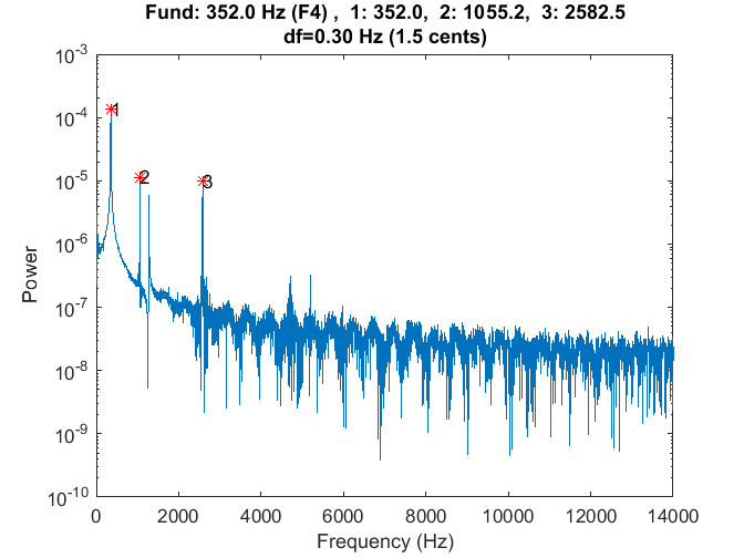
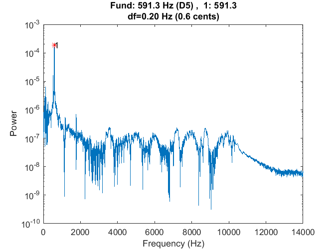
Another difficulty of bar tuning by using spectral analysis is related to the nature of wood itself; wood is only approximately homogeneous as its density varies throughout due to internal checks and knots. This variability can result in extraneous resonant modes that are identified by the spectral analysis. For example, consider the spectral plot at the top of this page. The software did a good job of identifying the first three partials and labeled them 1, 2 and 3. However, there also exists a mode just to the right of the second partial. This is real, and can affect the tonal characteristics of the bar.  These extra modes can sometimes confuse the software and make the plots a little messy, especially when producing “roll-up” plots that provide data for all notes. For example, here is plot showing the ratios of the partials that were determined by analyzing each note of the C major scale clip form the YouTube video:

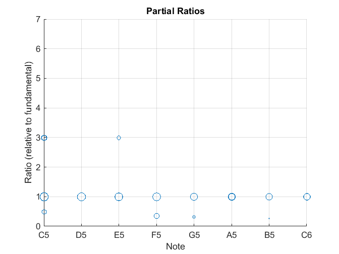
On this “ratio plot,” the note names are plotted along the abscissa, and the ratios of the measured partials are plotted along the ordinate. The note names are determined by finding the closest ideal note (based on a 442 Hz pitch reference) to each measured fundamental frequency. All data for a single note are plotted in the “column” above the note name, so if a particular note is contained multiple times in a sound file, this will result in little groups of points that are close together. The circle size on the plots relates to the power in the partial. (Actually, the size is proportional to the log of the power.) Typically, the larger circles represent modes that we care about, and the smaller circles correspond to low power extraneous modes that don’t affect the sound too much.

Spectral Analysis Challenges

You will notice some weirdness in these plots from time to time. As noted above, this is typically due to extraneous modes. For example, consider the first note from the C major sound clip. Here is the FFT for that note:

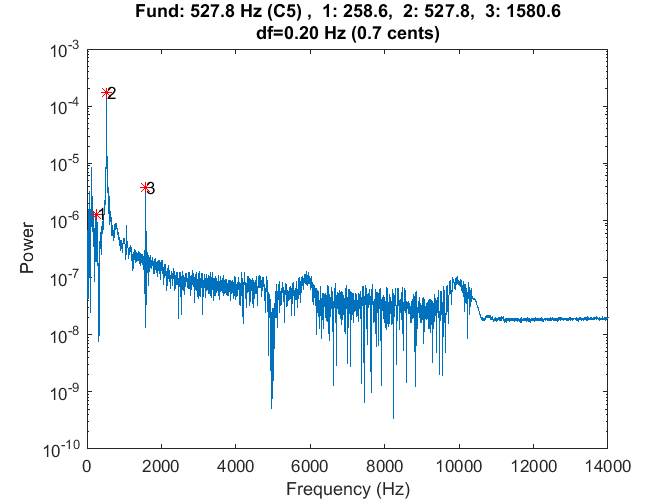
The software correctly identifies the two dominant modes, labeled 2 and 3 on the plot above, but it also finds another tiny mode that is below the fundamental frequency of the note. This may be real, it may be some artifact of the spectral analysis or it may be the result of poor sound fidelity in the YouTube clip. In any case, the result is the extra circle on the plot that has a ratio of about 0.5. In some cases, extra tones will appear that result from torsional modes in the bar (as described in LaFavre et al,) especially if the bar is not struck at the bar center.  The good news is that the software still correctly identified the fundamental (i.e., the major peak at 527.8 Hz) so that the ratios can be calculated correctly.

In addition to the extraneous modes, the other oddity that the the ratio plots will sometimes exhibit is missing modes. For example, in the ratio plot above, the software did not find a second mode for most of the notes. Here is the FFT for the first D5 note in the sound file:

The fundamental mode is easy to identify, but then there are some very small peaks later on in the plot that may or may not correspond to the second partial. The lack of significant peaks for the higher partials may be the result of the poor sound file quality, or it may be the result of where the bar was struck – I found that when the bar was struck “dead center,” the second mode was typically very weak and difficult to measure. You will here lots more about this later when I get into the discussion on bar tuning.

The “ratio plots,” like the one shown above, are useful because they quantify how well the instrument produces partials in the desired 1:3:6 tuning ratio. However, the ratios are normalized to the measured fundamental, so they do not quantify the absolute tuning accuracy of the instrument. Consequently, I produce a plot of the tuning accuracy for the fundamental mode like that shown here (again, for the C major sound file):

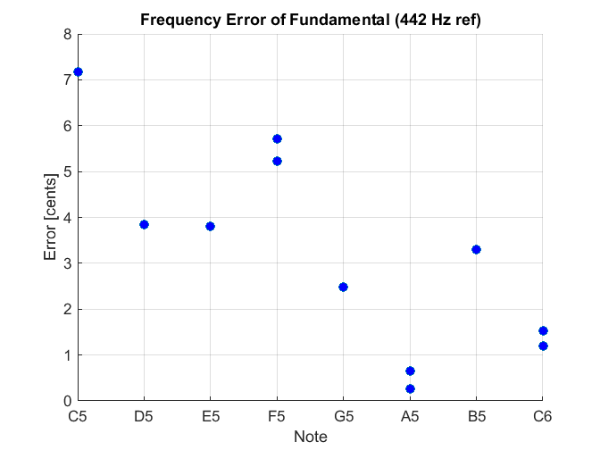
This “absolute tuning error” plot quantifies the error, in cents, for the fundamental frequency of each note. In musical parlance, the space between adjacent notes on an equally tempered chromatic scale can be broken up into 100 equally spaced intervals. Each of these intervals is called a “cent.” Mathematically, as previously noted, the interval between notes is given by the ratio 2^(1/12) ~= 1.0595. A cent is defined as the interval 2^(1/1200) ~= 1.000578. Because a cent is defined as a frequency ratio, the frequency interval corresponding to a cent varies with frequency. For example, a cent for the C5 note corresponds to a frequency delta of

FreqDelta = Freq_C5 * (1-2^(1/1200)) = 525.63 * 0.000578 = 0.304 Hz

In contrast, the frequency delta of a cent for the D5 note is 0.341 Hz.

The absolute tuning error plot presented above shows that the xylophone used to produce the C major sound clip was tuned a bit sharp for all of the notes of the scale. The C5 note was worse, at about 7 cents sharp. The A5 note, however, was almost spot on.

Finally, the Results

The above description is a bit verbose, but it is necessary to understand the results of the analysis for the various xylophones that were analyzed. The results of these analyses motivated the tuning approach of my own xylophone bars and I believe provide a unique and practical reference for those interested in quantifying the sonic performance of xylophones. In the next section, I will present the actual results of these analyses.