Tag Archives: tuning

Tuning the Tubes

The resonator tubes are an important part of the xylophone. They boost and shape the sound produced by the bars. There is lots of information on the web about resonator tubes, so I won’t repeat that, but I will discuss our approach to making, mounting, and tuning the tubes.

The Physics

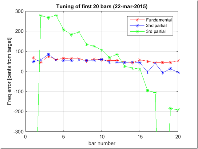
It is not hard to find info about “quarter wave stopped resonator tubes” on the web (in musical parlance these are sometimes called “stopped pipes.”) This is the type of resonator tube that is used for xylophones and marimbas These tubes basically resonate at a fundamental frequency of c/4L, where L is the length of the tube and c is the speed of sound. In simple terms, the tube boosts the bar sound amplitude by utilizing the normally wasted downward-directed sound energy in a way that boosts the upward facing energy (which is what you mostly hear). It shapes the sound too, because it does not boost all frequencies equally. In particular, it only boosts the fundamental and the odd harmonics. Because xylophone bars are tuned to a 1:3:6 frequency relationships, the fundamental and second partial will be boosted, but the third partial will not. This is another reason why I wasn’t too concerned about tuning the 3rd partial – its already puny energy is swamped by the boosted energy of the first two partials. Additionally, while we haven’t discussed it much, real xylophone bars “ring up” not just the “transverse modes” that dominate the sound, but also lesser “longitudinal” and “torsional” modes. Because these modes are not typically odd harmonics of the fundamental, they do not get amplified. So, at the end of the day, when tubes are added to the instrument, you mostly hear the fundamental and the second partial – all the other frequencies get dwarfed.

Tuning the tubes is done by adjusting a movable stopper that effectively changes the length of the tube. This is what determines the length L in the equation above. So you might think that tuning the tubes is just a matter of computing the tube length via the equation above and then setting the stopper to that length (I did,) however, like most equations from physics, the formula above is only approximate. It is very accurate under certain conditions, such as when the tube length to diameter ratio is large and the sound input to the tube is a “plane wave.” However, neither of these assumptions is true for the xylophone. In particular, the shorter tubes have a relatively low length-to-diameter ratio; and the sound wave coming off the bar is likely not planar, since the bottom of the bar is curved.

Dr Entwistle pointed me to a book called “The Physics of Musical Instruments,” by Rossing and Fletcher (ISBN-13: 978-1441931207,) that had some interesting comments about xylophones and ¼ wave resonators. In the section on resonator tubes, they note that the resonant frequency of the tube is a weak function of the distance between the tube end and the bottom of the bar. However, they state that “As yet, the theory describing the coupled bar-resonator system has not been worked out in detail,” which basically means that there is not a simple equation to compute the actual stopper position as a function of the desired frequency.

Additionally, the Rossing book describes a few topics of practical importance. First, the it describes something referred to as the “end correction factor.” It turns out that the equation above must be tweaked somewhat due to the fact that the standing wave in the tube does not end exactly at the pipe mouth but is rather a bit beyond it. The more accurate equation for the resonator frequency is f =c/[ 4(L+0.61r)], where r is the radius of the tube. I found other references to the end correction online and there appears to be some debate in the literature over the correct value of the correction factor (i.e., the value of 0.61).

As noted above, the book notes that the tube frequency is affected by the spacing between the tube end and the bar bottom. I had already seen that some xylophones allowed for adjustment of the height of the tube assembly (i.e., the assembly of all of the tubes locked together into a rigid structure) to compensate for temperature changes. It makes sense that if the tube-bar spacing is less than the 0.61r factor, then it will affect the tube resonance since the bar is effectively serving as a stop at the top of the tube.

At the end of the day, it became clear that the bars must be tuned in situ to obtain accurate tuning. However, I couldn’t resist the urge to check out the physics, so I did a few experiments and built some tuning curves that I hoped might at least guide the resonator tuning. However, in the spirit of full disclosure, I must note that I mostly ignored the results from this effort and just tuned the tubes by ear! Nevertheless, I will describe these experiments, if for no other reason than to perhaps save others the folly of this endeavor. You can safely skip this section without regret if you just want to git-er-done…

Tuning the Tubes

I started out by doing experiments with a piece of PVC as I awaited the delivery of the aluminum. I was particularly interested in verifying the resonant behavior of the tubes as a function of spacing distance to the bar. It wasn’t clear to me how to establish the correct tube-bar spacing. Intuitively, it seemed to me that the best coupling might result from close spacing, so that the spacing would be dictated by physical constraints, like avoiding contact if the bar should sag.

In order to start my experiments, I needed a value for the speed of sound. The speed of sound is a function of the density of the air, which is a function of the temperature. I found an online calculator here that computed the velocity. During my experiments, I measured the temperature at 19.2 C, and the the online calculator gave me a velocity of 343 m/s.

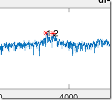
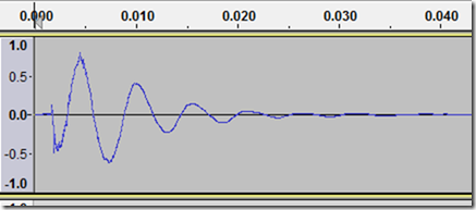
I must admit that I struggled a bit with how to find the resonant frequency for my PVC resonator pipe. I fabricated an adjustable stop and set it to yield a 15.0 cm tube. Per the standard 1/4 wave calculation (with a 0.61*r end correction,) the computed frequency was about 525 Hz. I experimented with several methods of exciting the bar. I tried whacking the end of the tube, and attempted to measure the impulse, but the resonance died out rather quickly. Here’s an example where you can see that the pulse dies out in about 25 ms:

Measured decay of 15 cm tube after being whacked.

I did some decayed sinusoidal fitting to this, but wasn’t able to get accurate results. Ultimately, I used a small speaker to excite the tube as shown in this photo:

PVC tube with small speaker used for excitation

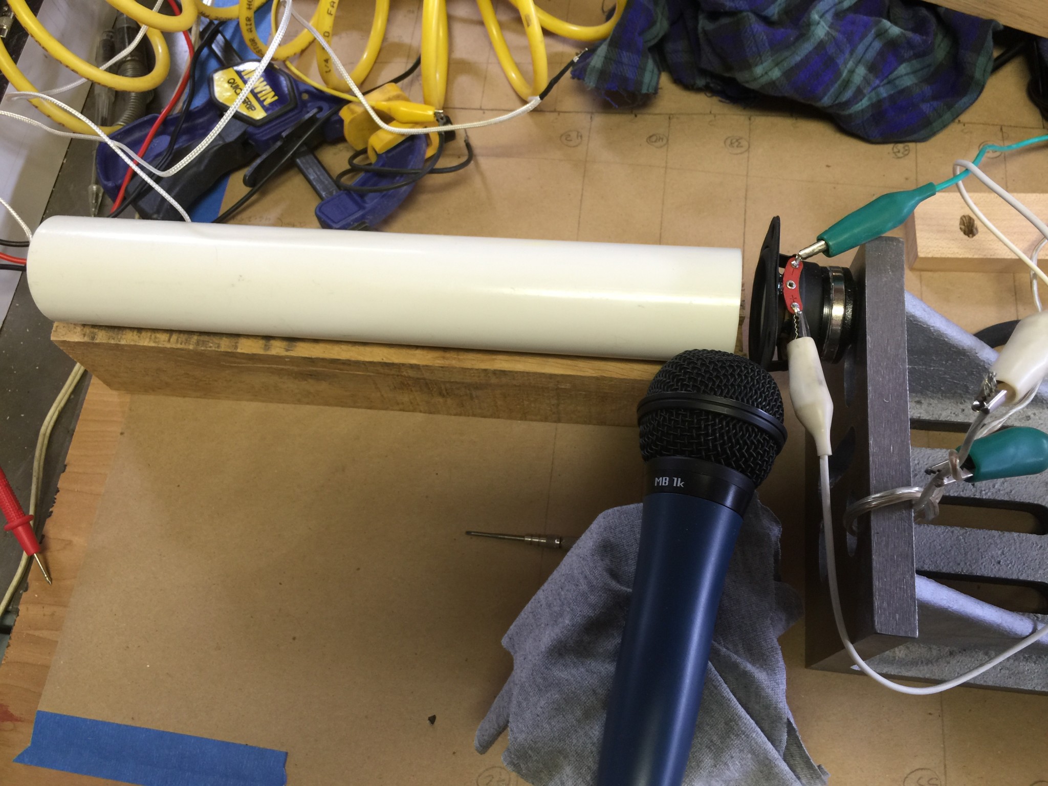
The tube was excited by the speaker at the right, and the resulting audio was recorded with the microphone.

Next, I tried exciting the tube with white noise. Interestingly, you could easily hear the “coloring” of the noise due to the modes. This gave PSD plots like this:

PSD of white noise response.

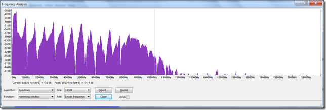
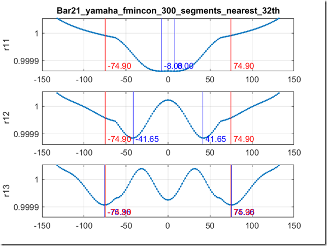
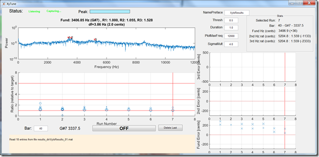
However, I found that identifying the peaks was unreliable. Ultimately, I wrote some Matlab code to generate and play a frequency sweep while recording the response. Here is an example of one of the PSD curves:


PSD of 15 cm tube excited with frequency sweep.

This is what the recording sounded like for this tube:

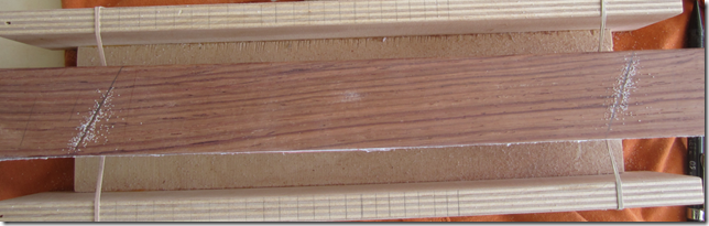
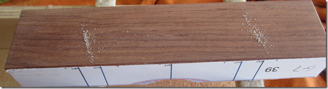
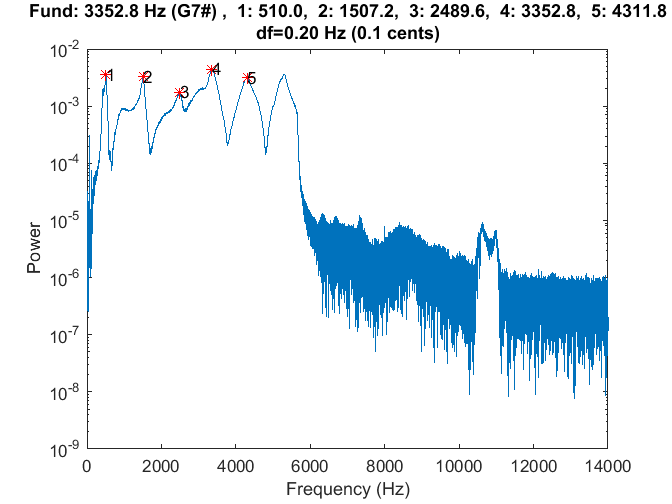
The code identifies the peaks (which of course correspond to odd harmonics). However, the first peak (the fundamental) was always a bit broad and had a sort of “shoulder” to it, which made me doubt it. So I wrote a little algorithm to find an the optimal “least common factor” for all of the identified peaks. The higher harmonics had generally broad peaks so I also ignored them, and only used the lower modes. In general the setup was somewhat fickle and the quality of the peaks that I got was a strong function of the microphone and speaker placement. In any case, here is some data for my 15 cm tube:

Temp = 19.2 deg C


>> ResonatorTune(500, 'res=15.0, spc=3.0')

res=15.0, spc=3.0 -

Fund: 509.0

, Error (Hz): 5.9, NumModes: 2

   Mode 1: Error (Hz): +10.6

   Mode 2: Error (Hz): -1.2

>> ResonatorTune(500, 'res=15.0, spc=2.0')

res=15.0, spc=2.0 -

Fund: 509.4

, Error (Hz): 6.0, NumModes: 2

   Mode 1: Error (Hz): +10.8

   Mode 2: Error (Hz): -1.3

>> ResonatorTune(500, 'res=15.0, spc=1.0')

res=15.0, spc=1.0 -

Fund: 505.0

, Error (Hz): 2.8, NumModes: 2

   Mode 1: Error (Hz): +5.0

   Mode 2: Error (Hz): -0.5

>> ResonatorTune(500, 'res=15.0, spc=0.5')

res=15.0, spc=0.5 -

Fund: 492.5

, Error (Hz): 3.4, NumModes: 2

   Mode 1: Error (Hz): +6.1

   Mode 2: Error (Hz): -0.7

These data correspond to 4 different collections with varying standoff distances from the end of the tube to the speaker (from 3.0 cm to 0.5 cm). It is interesting that the frequency doesn’t shift above about 2 cm, but there is a nearly 20 Hz shift when the tube is very close to the speaker. This clearly shows the behavior noted in the Rossing book (i.e., decreased frequency for close spacing,) which was pretty cool.

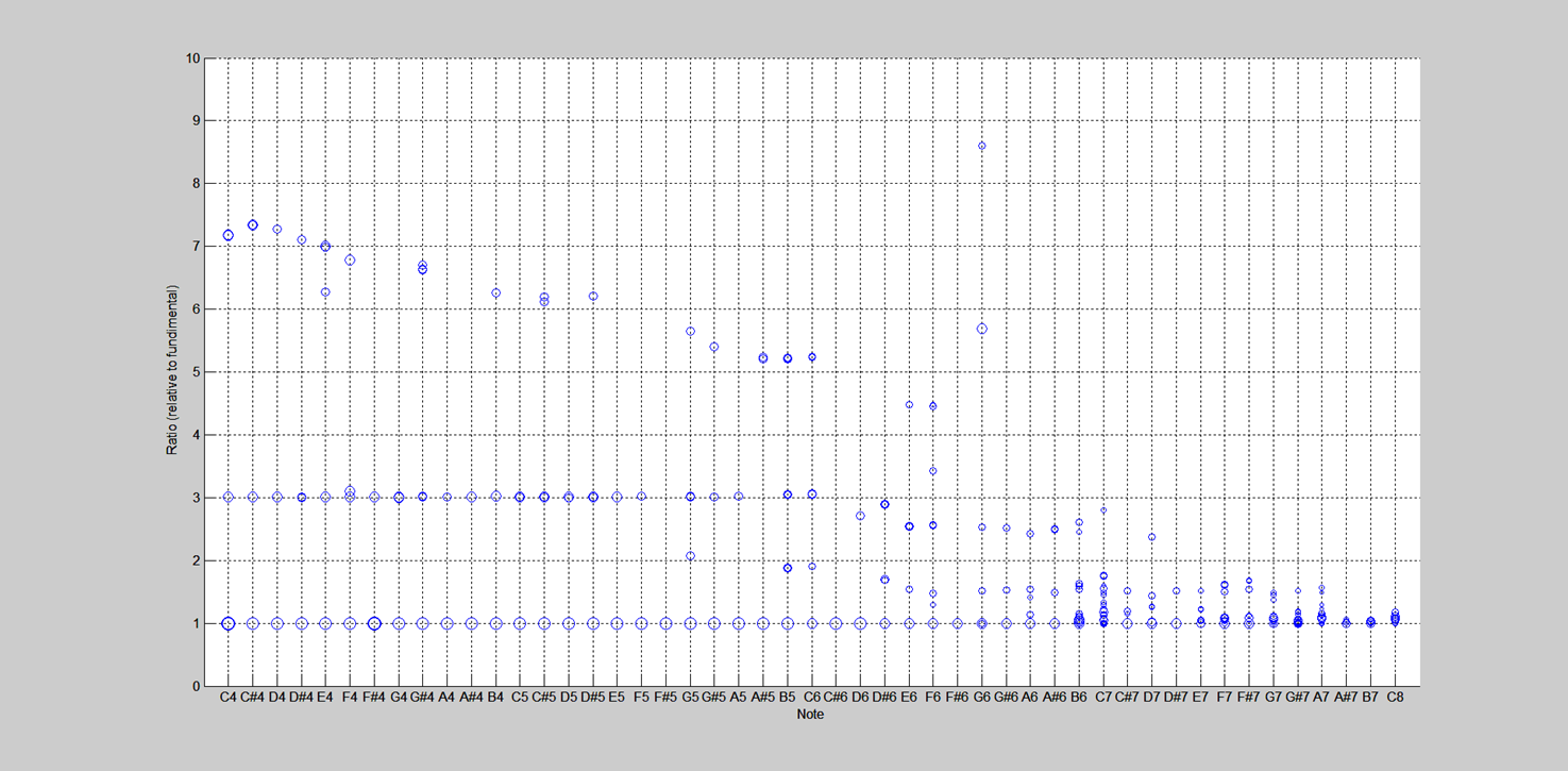
So using this technique, I set off to build a curve that could be used to set the stopper distance for each tube. I chose to set the distance at 0.5 cm, which is about as close as I could safely space the tubes from the bars without fear of contact. For each stopper distance, I performed a sweep and used my least-common-factor code to find the tube resonance. With this approach, I was able to build the following curve.

Resonator tube tuning curve.

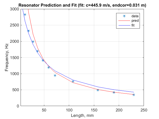
The blue points on the curve are the measurements and the red line was created using the frequency equation given above (including the 0.61r end correction factor). The equation accurately predicts the frequency for the longer pipes, but performs poorly for the short pipes. As a quick test, I tried fitting the equation above, but left the speed of sound and the end correction factor as free variables. This resulted in the blue curve. The fit was better for the short tubes, but resulted in poor performance for the long tubes. So I decided to skip function fitting entirely, and just set my stopper distances by interpolation between the measured points.

Next Up

This post described some of the science involved in establishing the tube resonant frequency. In the next post, I will describe the fabrication and mounting of the resonator tubes.


Drilling the Holes

The last lengthily post described the method and results for the rough tuning of our 44 bars and described a few challenges that we encountered along the way. Here we are going to describe the process of determining the suspension hole locations and the actual drilling.

To simplify construction of the xylophone, it would be best to have the cord that suspends the bars follow a straight line; this allows straight support rails and straightforward placement of the suspension posts. Also, all of the commercial instruments that we inspected were built with straight suspension cords.

Having measured all of the node locations using the salt method, we were able to assess how linear the node locations were and how much they would deviate from a straight line. The next plot shows these results.

Hole locations with linear trend lines

The symbols are the measured node locations from the front and rear ends of each bar (we define “front” to be the bar ends that face the player). There is clearly a gentle deviation from linear, but it is modest, so I chose to ignore it. Doing otherwise would force me to mount the suspension posts along a curve, which would obviously complicate construction.

Of course, the holes must be drilled at an angle relative to the bars. To figure out the hole angles, I wrote a little code to plot the locations (as if you were looking down on the instrument). I left 1/4 inch spacing between the bars, which might be a little tight for mounting posts, but I can space them a bit more later if needed (this, of course, affects the angle slightly, but the change is negligible). The following figure shows the output of this code.

Bar and hole locations

There is a lot going in this figure, so let me explain. The plot basically shows the location of the bars’ ends and posts in physical space. The blue solid lines show the locations of the natural bar ends. The red lines give the same info, but for the sharp bars (also called the accidentals). As you can see, the front edge of the sharp bars overlaps the back end of the natural bars. This is allowed, as the rear bars are elevated. In general, it is desirable to have the accidental bars as far forward as possible to minimize the reach needed by the player. The asterisks show the measured node locations for each bar, and the dashed line is the best linear fit through the node locations. If you look carefully, you will note that the solid lines (the bar end locations) are a bit wiggly. This is because I shifted each bar for and aft (actually Matlab did it) to split the difference between the best-fit line and the node locations. I did this to minimize the distance between the linear fit and the true node locations. Aesthetically, this is somewhat undesirable (i.e., the bars ends are not perfectly lined up,) but results in more bar sustain, since the damping due to the mounting string is minimized.

The hole angles that I computed from Matlab were

Natural front hole angle (deg): 10.4
Natural back hole angle (deg): 2.3
Sharp front hole angle (deg): -2.2
Sharp back hole angle (deg): -10.5

Jack and I started marking all of the computed node offsets on each bar, but this got pretty tedious. In the end, we laid them out carefully on a piece of craft paper that had markings for the horizontal locations and then empirically adjusted the bars to get the best fit to a straight line. Here are a bunch of photos showing the layout and alignment to the penciled node locations:

The yellow thread was stretched between two posts to establish a perfectly straight line. As noted above, we visually scooted each bar to try to minimize the distance between the yellow thread and the penciled node marks. When we got them sufficiently aligned, we laid down a 4 foot straightedge aligned with the thread and marked the compromise hole locations on each bar.

Finally, at the top of the page is a picture of the drilling operation. We faced a 90 degree cast iron angle block with a piece of 3/4 inch melamine that had lines for the 2.2 deg and 10.5 deg marks drawn on it. We clamped on a stop block aligned with the marks to keep the bar from sliding down the melamine as the holes were drilled. For the 10.5 degree holes, we used a center drill to start the holes to avoid bit wander and then finished the holes with a 3/16 inch drill bit. Here is a photo of all of the bars with the drilled holes:

All bars with drilled holes

The red lines near the holes of each bar correspond to the computed node locations. The agreement is between these computed locations and the drilled hole locations is generally quite good.

In the next post, we will move forward with the fine tuning after which we will have almost completely finished bars!

Rough Tuning 44 Bars

In the last post, Jack and I turned all of our blanks into shaped bars by cutting and sanding a bit proud of the computer-generated profile line. Now we had to “rough tune” them in preparation for drilling the suspension holes. I had previously noted that drilling the holes had almost no effect on the frequencies for our maple test bar. However, I did a quick test on a much shorter bar and found a significant “flattening” of the fundamental mode. We decided to rough tune each of the bars to about 50 cents sharp to pre-compensate for the hole drilling.

Temperature and Humidity

In our correspondence, Dr Entwistle and I speculated about the affect of temperature and moister content on the sonic properties of the bars. Rodney suggested that perhaps friction heating resulting from the drum sander might affect the spectral measurement. This was a good point, so I decided to do a quick temperature sensitivity experiment.

First, I took one of my prismatic Rosewood bars and measured the spectral characteristics at room temperature to establish a baseline. The fundamental was at 1868.0 Hz at a thermal equilibrium temperature  of 18.1 C. I let it soak in the fridge overnight, and measured the cold temperature at 1.0 C. I then removed the bar from the fridge and quickly measured the fundamental to be 1884.8 Hz. I was surprised that the frequency didn’t change more. This is only about a 0.9% change (15 cents) for a 17 deg decrease or about 1 cent/deg. This result was good news, because it suggested that I did not have to worry too much about bar heating during the tuning process.

Moisture content was a different story. The process of developing the tuning process, and the mechanics of tuning 44 bars took months. I purchased the Rosewood in January of 2015, and finished the tuning in October – about 10 months. During this period, I noticed a consistent pattern; whenever I left weeks or months between spectral measurements, I would notice a significant sharpening of the bar frequencies. I suspected that this was due to wood dry-out over time. You may recall me noting that the vendor who provided the wood stated that he had recently received the shipment of Honduras Rosewood – it had not been in Albuquerque long prior to my purchase. I can only speculate where the wood came from, but it is likely that it was from a climate that was more humid than the arid desert of Albuquerque. New Mexico has a typical relative humidity that is typically 10 or 20%, so we are more dry than just about anywhere.

When I first got my Rosewood in January, I measured the density of a couple of prismatic test bars. To establish the density, I weighed the bars and accurately measured the dimensions. This yielded the following densities.

January 2015
rho1 = 1081.7 kg/m^3
rho2 = 1082.1 kg/m^3

Just today I re-weighed the bars and re-calculated the densities as

February 2016
rho1 = 1042.4 kg/m^3
rho2 = 1041.9 kg/m^3

This is about a 4% decrease in density over 13 months. Wow! This will certainly have an affect on the bar frequencies.

I guess the lesson is that one should properly season the wood to their local climate prior to tuning these bars. (Anectodally, Dr Entwistle suggested letting the bars acclimate for a year or so prior to shaping them, but I was just too eager to get to cutting!) In any case, I lucked out in that the bars got sharper, rather than flatter over time. Recall that it is much easier to decrease the modal frequencies than it is to increase them. This would have been a serious mistake if I lived in a more humid climate, such as Florida. This is another big “lesson learned” for those of you out there who may be attempting to build your own instruments.

Back to Tuning…

First, we re-cut the three bars that were sonic outliers. This was not a big deal, but did involve all of the familiar steps (ripping, planing, jointing, sanding, etc.). It’s so much faster the first time when you are doing it in volume! We also printed new labels and got them adhered to the bars. The frequency response on these new “blanks” was in family with the bars around them, so we were comfortable moving forward with shaping.

In our first run at tuning, we got 20 done. We were shooting for about 50 cents sharp on both the fundamental and first partial. The graph below shows the current state of our first 20 bars.

Modes for the first 20 rough-tuned bars.
Modes for the first 20 rough-tuned bars

As you can see, the first and second partials are well behaved for most of the bars. The third partial, which we decided not to tune, wanders around similarly to other xylophones that we had  spectrally measured.

Note that as the bars got shorter, the computer-generated bar shape became less accurate. As you can see on bar 16, 18 and 20, the second partial is tuned about perfectly (not 50 cents sharp, as targeted). This is not due to my tuning, but rather because the second partials for these bars were already closely tuned directly after band-sawing the shapes ~2 mm proud of the computed profile. To tune these bars, I removed wood only at the center of the bar to minimize the affect on the second partial. As you can see in the following photo, these bars shapes have deviated quite a bit from the computer prediction.

First 20 rough-tuned bars

Over the subsequent weekend, Jack and I were able to get the rest of the bars tuned. Here are the tuning results:

Frequency characteristic of all rough-tuned bars

The fundamental on all bars was pretty good except for bar 29 (my A6 bar,) on which I must have daydreamed while sanding, thus making it a bit flat. I thought that I might need to fix that bar, but that turned not to be the case since the moisture dry-out sufficiently sharpened the bar prior to fine tuning. The second partials above bar 21 (C6) were mostly flat even with the +2 mm rough sawing. However, I was not concerned, because this is consistent with other xylophones that I measured. For example, here is the tuning for the Kori xylophone  that I measured:

Measured spectral tuning graph for Kori xylophone.
Measured spectral tuning graph for Kori xylophone

As you can see, for the bars above C6 the second partials for this xylophone are whacky or too quiet to measure.

Here are photos of all of the bars, rough tuned:

Rough tuned bars 1-10
Rough tuned bars 11-20
Rough tuned bars 21-28
Rough tuned bars 23-31
IMG_3589
Rough tuned bars 32-44

The photos show that, starting at bar 18, I had to cut a very narrow notch at the center to yield the desired tuning. As noted above, this is because the rough-sawed shape already had a second partial that was close to the +50 cents desired. As I’ve said previously, the computer predictions start to break down for the shorter bars (as a point of reference, bar #18 is about 11.5 inches long). I don’t think that this is due to inconsistency with a single bar, because the issue seems systematic for all of the “shorter” bars.

Another limitation that I found with the computer results concerns the tuning curves. For example, here is the tuning curve for bar 21:

Tuning curve for bar #21

This curve shows a subtle sharping of the 2nd partial for wood removed at the center. The trend gets more pronounced for the shorter bars. However, I saw no evidence of this when removing wood at the center. I typically saw no change in the second partial with wood removed from the center. As I’ve discussed previously, all of this is likely just a limitation in the approach (i.e., bar theory).

An Improvement?

Later, after doing all of the rough tuning, it occurred to me that I could have modestly improved on my approach to the computer predictions. Specifically, since I performed frequency measurements for each of the Rosewood blanks, I could have used these to compute the modulus for each bar. I could have used this, plus the measured densities for each bar to compute the bar shape for each bar’s paper template. (Recall that I used a single average modulus value and density for all bars.) While I am guessing that this would have reduced variability between the predicted and measured bars, I doubt that it would have significantly improved the systematic issues I saw with the short bars which are most likely the result of the “plate-like” geometry of the shorter bars. Nevertheless, using the per-bar modulus and density seems like a better approach and one that I would recommend.

Wrapping Up the Rough Tuning

Because the computer predictions only approximate the nodal locations for bar, Jack and I used the “salt method” to determine the actual node locations. Here are a few photos. First, is a photo of the salt results for a long bar, including the pencil marks I drew through the salt “mounds.”

Salt test results for a typical long bar

Here is one of the shorter bars, before and after strikes with the mallet:

Salt sprinkled on short bar (prior to mallet strikes)
Salt test results (after mallet strikes causing salt to migrate)

The salt results for bar #40 were curious – the nodes did not form lines at all, but rather fairly circular clusters as shown here:

Salt results for bar #40

This one also had an atypical spectrum, as shown here:

Unusual spectrum measured for bar #40
Zoom of bar #40 spectrum

The zoomed plot shows that there were two modes that were very close together.  Compare this to bar #39, which was typical of the spectrum for most of the short bars.

Zoomed spectrum for bar #39 showing typical results

Bar #39 shows a nice, single discrete fundamental mode.

Dr Entwistle suggested that perhaps the two close modes that were were observing with bar #40 was the result of a torsional mode closely coinciding with a bending mode. We spent a bit of time trying to ring up the torsional modes to test this theory, but found it difficult. The La Favre site showed some torsional mode results, but that was for marimba bars which are substantially wider.

Bar #40 definitely seemed like an outlier. It also sounded a little different than the others – perhaps a little less “bright” than its neighbors. Jack and I considered remaking this bar, but in the end, decided that it wasn’t worth the effort, given the subtle effect.

The Sound

Here is a sound file containing all of the rough-tuned bars:

A few notes on this sound file:

  1. The mallet double-bounced on some of the strikes, which you can hear.
  2. You can hear a “warbling” for the first few bars. This is due to the Doppler effect that result from the bar bouncing on the rubber-bands of the tuning jig after the bar is struck. As an aside, this warble is perhaps a few Hz so I later wondered if it could be broadening my spectral peaks and reducing the accuracy of my spectral measurements. A modification of the tuning jig that utilized e.g., felt strips rather than rubber bands would have addressed this potential issue.
  3. You may also be able to hear the flat A6 bar.

Having rough-tuned all of the bars, I guess if I were going to do this again I might do some sanity checks along the way to identify anomalous bars early to avoid unnecessary work. For example, after cutting each bar to length, but prior to sanding, attaching the label, or rough-cutting the under-shape, I would probably do a quick spectral check and do the salt method. Then, I could reject any bars that were out of family with the rest. For example, I would check for:

  1. A fundamental or second partial out of family with the rest
  2. The double peak in the fundamental (like my bar #40)
  3. Out of family salt results (i.e., weird nodes)

This quick up-front work could save some considerable re-work down the line.

As a teaser, here is a photo of our 44 bars in an approximate lay out. Pretty cool to see it becoming an instrument!

Rough tuned bars laid out in there approximate configuration