In the previous post, I described the math and software used to compute the undercut shape for a maple test bar. That was step 1. In this post I will describe step 2, which is actually cutting the bar out of wood.
Making the Bar
The first step in the process is cutting a piece of maple to the correct dimensions. I selected a piece of boring, straight-grain maple and cut it to the dimensions of the Yamaha F4 bar. After cutting, I measured the bar to record the exact dimensions:
Length=15.05
Width=1.502
Thickness=0.875
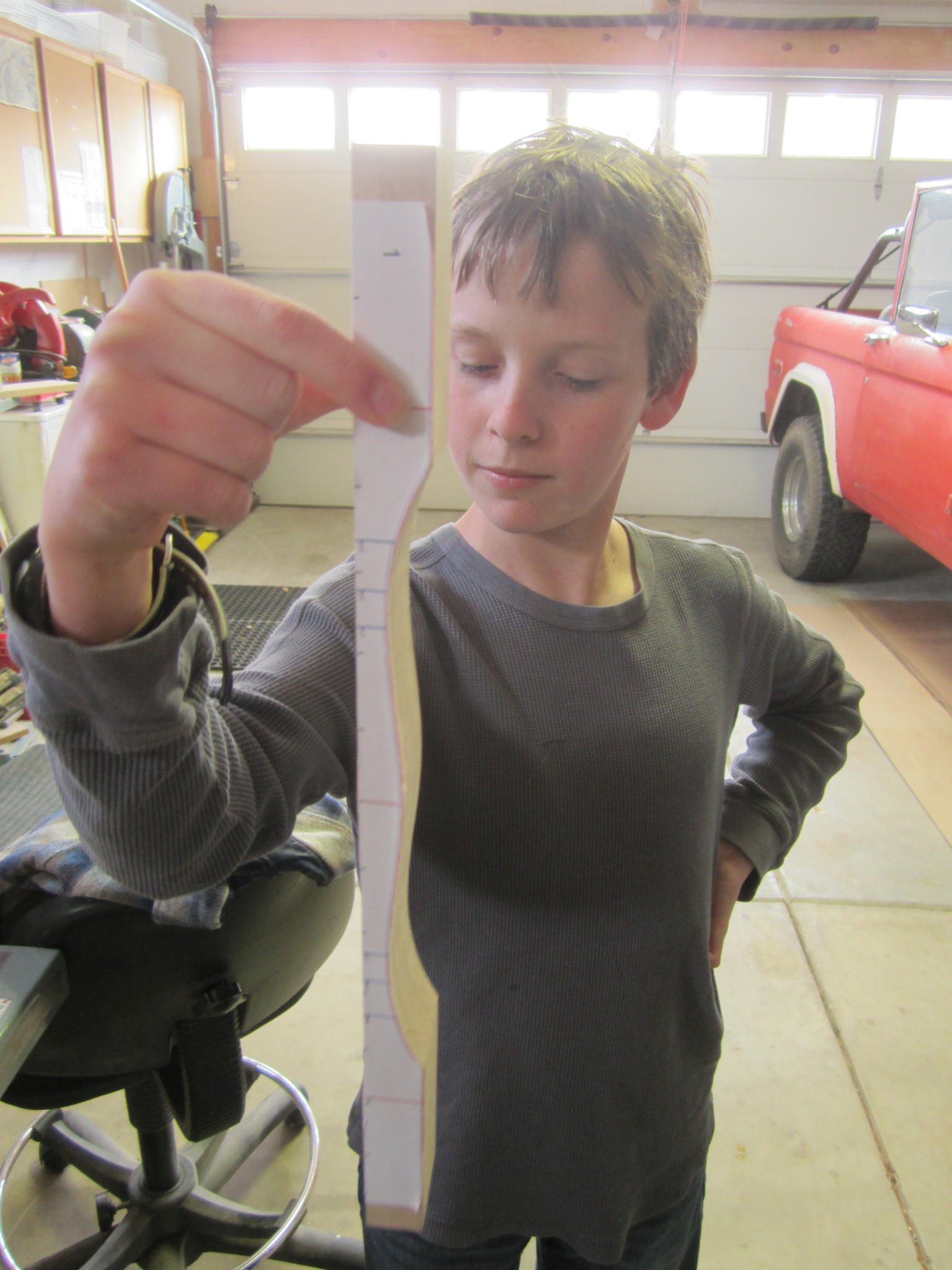
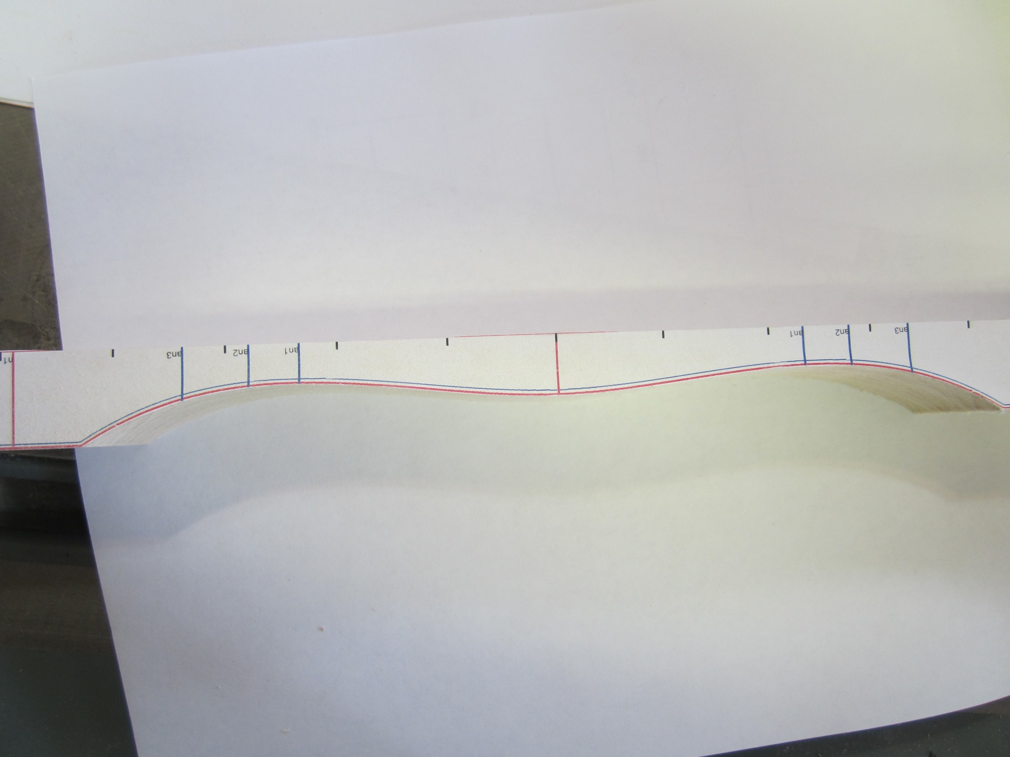
In order to shape the wood so that it conformed to the computed shape, I printed a full-scale paper template directly from Matlab. I’ll spare you the mundane details, but it took some trial and error to get Matlab to print precisely in full scale and to compute a calibration factor for the printer. Here is the template that I made:

There are lots of lines on this bar, so let me elaborate a bit. The first thing you might notice is that there are multiple profile curves. The red curve is the cubic that the software computed. The other curves are included as index lines, so I could precisely determine how close I was to the red line as I was cutting the wood. They are spaced exactly 1 mm apart.
There are multiple vertical lines that warrant description. The vertical red lines labeled “n1” were intended to mark the locations of the nodal points (aka nodes) of the fundamental vibrational mode. However, I will discuss later that this location is incorrectly marked – the actual nodes are over 1 cm away from these lines. The other vertical lines, marked an1, an2 and an3, were intended to locate the anti-nodes of the higher modes. Anti-nodes are the location where the bar deflects maximally in the transverse direction (i.e., perpendicular to the long axis of the bar). However, this terminology is erroneous – while these lines do correspond to a useful physical fiducial, they do not mark the anti-nodes. I’m afraid we have to go back to the vibration theory to flesh this out further.
“Tuning Curves” and Such
LaFavre and pretty much all of the papers do a great job discussing the vibrational modes of wooden bars. For each longitudinal mode, there is a point about which the bar bends. At this location, the bar exhibits no up and down motion as it vibrates. This fact is critical, and practical, in that it dictates the location of the mounting points for the bar. Theoretically, one could clamp the bar rigidly at exactly this point and there would be no damping of the bar due to the clamps. In practice, xylophones and marimbas suspend the bars on a string that passes through holes that are centered on the nodal locations in an attempt to minimize damping due to the suspension strings. My “n1” markings on the templates were intended to be the nodal locations of the fundamental, but were rather marking an important fiducial determined by “tuning curves” that I had computed. Let’s talk a bit more about the tuning curves, since these are critical to actually tuning the bars.
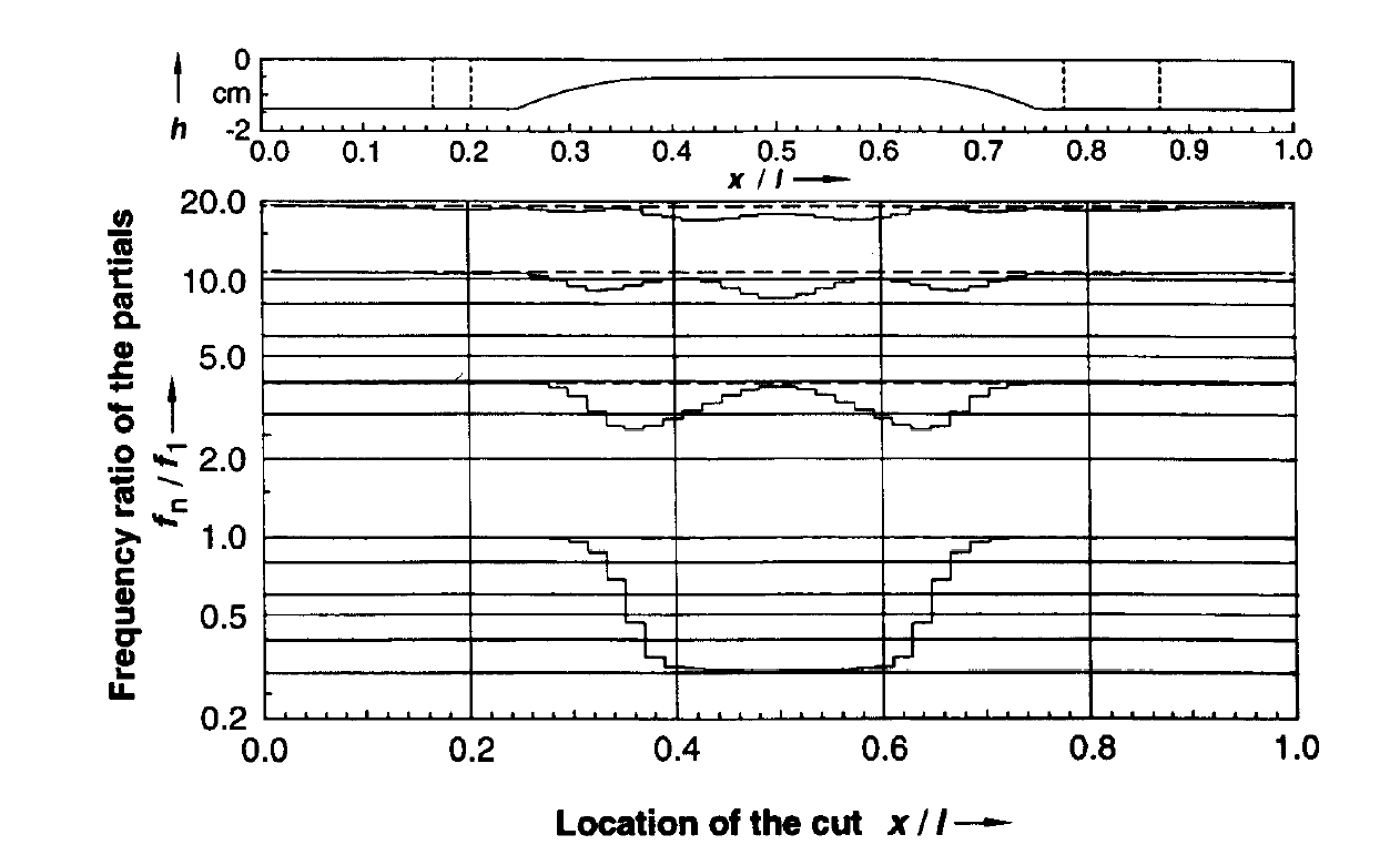
If you look back at Bork’s original paper (cited earlier), you will see plots that look kind of like this one:
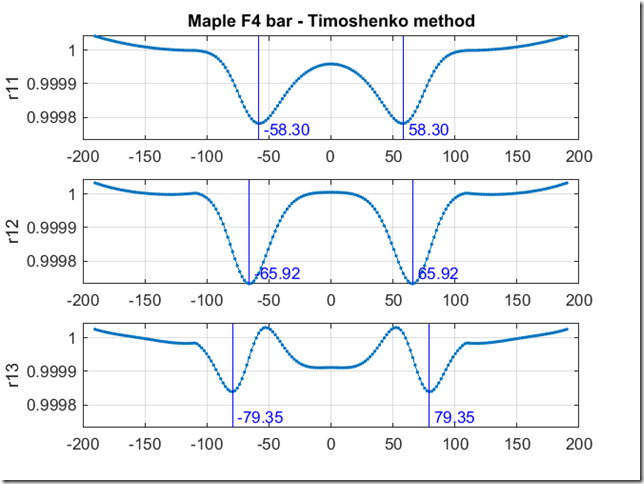
This is an example of what I call a “tuning curve” plot, which was created by basically following Bork’s approach. These curves quantify the effect of removing material from the bar at various points along its length. Consider the top plot first. On the y axis, I am plotting the ratio between the unmodified fundamental frequency (i.e., the bar frequency prior to removing material) to the fundamental frequency that would result if I removed a very small amount of material at various points along its length (as plotted along the x axis). By inspection of the plot, the curve shows that the most effective way to “flatten” (reduce) the frequency of the fundamental mode is by removing material at the at the locations denoted by the two vertical lines. The middle plot shows the effect of material removal on the second mode, and the bottom plot shows the effect on the third mode.
Why is this curve important? Well, as the Bork, Zhao, and other papers note, the math that determines the bar shape only gets you part of the way to a perfectly tuned bar. This is due to limitations of the math and assumptions that we make about the wood that are not completely accurate (e.g., homogeneity, isotropy, etc.). These curves are used during the bar shaping process to tweak the frequencies of the various partials. So the steps to tuning are:
- Compute the bar shape using the math.
- Fabricate a bar per the computed shape, but cut proud of the computed thickness profile.
- Measure the frequency of the partials.
- Consult the tuning curves to determine where to remove wood.
- Remove a tiny bit of wood at the indicated locations.
- Repeat 3-5 ad nauseam (or at least until the bar is sufficiently tuned).
In step 2 above, the word “proud” is taken from the woodworking vernacular and means making a cut that is bit thicker or wider or longer than the final desired dimension. In this case, we cut a little proud so that we have extra material to remove as we are tweaking the bar tuning – it’s much easier to remove wood than to add it…
The tuning curve above illustrates some very important facts about bar tuning. First, notice that the most sensitive way to make the fundamental flatter is to remove wood at +/- 58.3. Removing wood at +/- 65.9 is the fastest way to flatten the second partial. Importantly, notice that there is large overlap of the curves for the first and second partials. This is unfortunate, because it means that removing wood in this area of the bar affects both the first and second partials simultaneously, making it difficult to independently tuning the partials.
However, all is not lost. Looking carefully at the curves, you can see that removing wood from the very center of the bar weakly flattens the first mode, but has negligible affect on the second partial. Bingo – we have a way to independently tune the partials! Notice that this finding is consistent with Bork, and indeed he suggests the following tuning approach that we basically followed:
- Carefully remove wood from the region around +/- 60 mm until the second partial is about right.
- Remove wood from the bar center until the fundamental is perfect.
The tuning curves whisper one final secret to tuning. Notice the slight sharpening that occurs in all three modes when wood is removed from the ends of the bar? Well, this characteristic can be exploited if too much wood is inadvertently removed from the mid-portions of the bar. Here is another photo of the bars from the Kori xylophone I checked out.
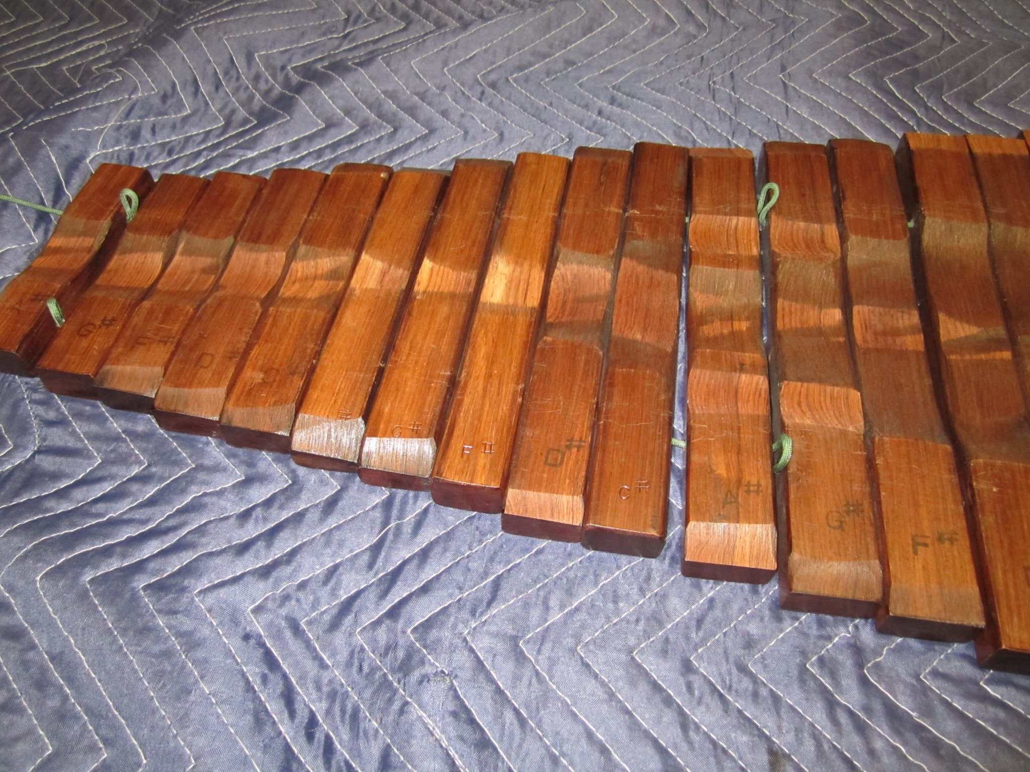
Notice that some of the bars have “chamfers” at the ends? This is presumably to sharpen the bar modes.
In general, I would suggest caution when exploiting this sharpening trick; as the tuning curves illustrate, and my experiments supported, the frequencies change is a very weak function at the bar ends; a great deal of wood must be removed to appreciably sharpen the bar.
Apologies are in order for the epic discussion above, but do feel that it is necessary to really understand the underlying motivation for the hands-on tuning of the bars. Your reward for staying with me thus far is the following section where I actually cut the bar (really, no bait-n-switch this time!)
Making the Bar (No Kidding)
February 15, 2015
As I mentioned above, I printed a paper template of the computed bar shape and attached it to my hunk of maple. Here is a photo of the bar with the template attached.
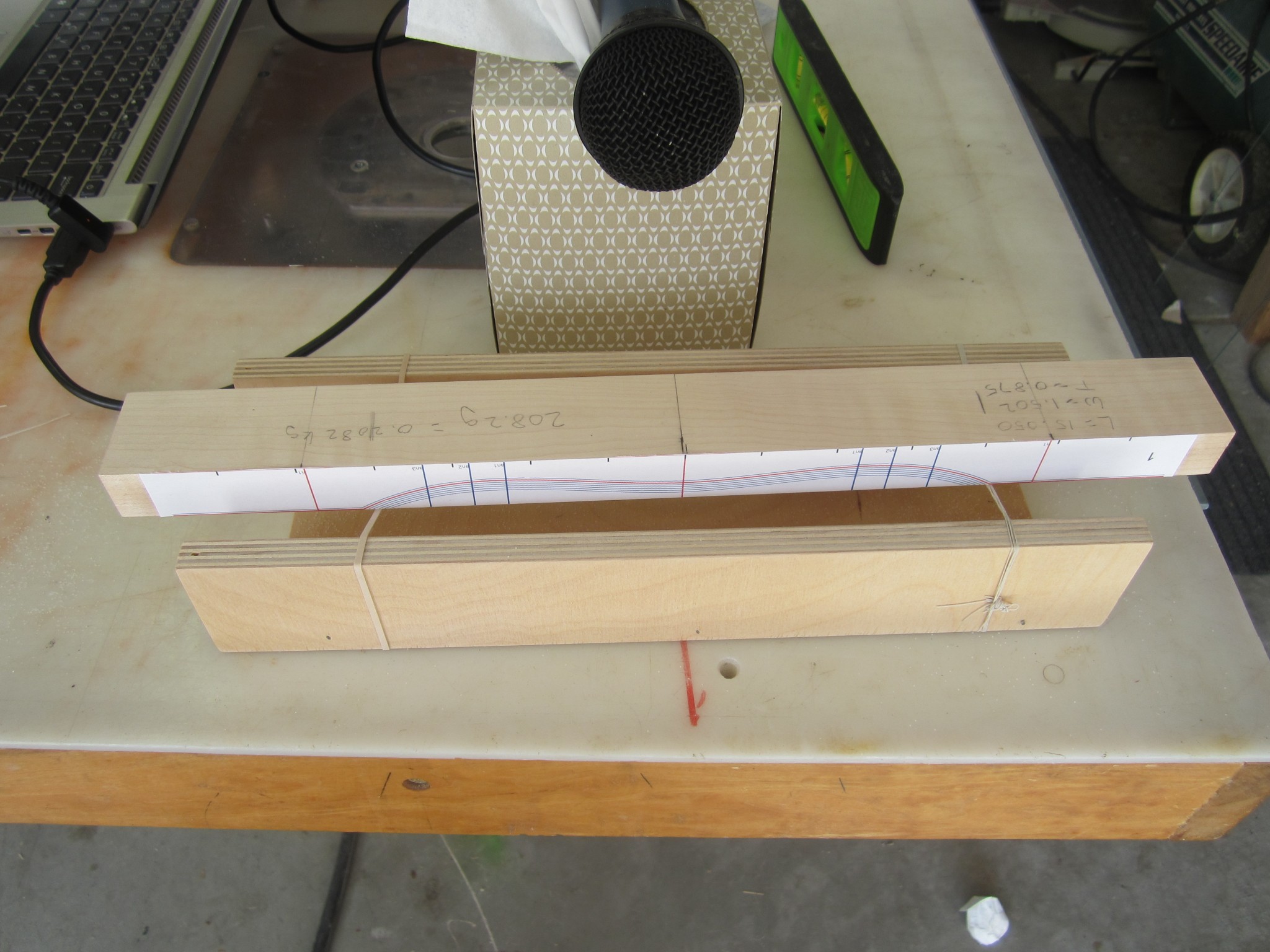
At the top of the photo you can see a microphone sitting on its mount (a Kleenex box). The microphone is connected to a computer so that when the bar is struck, the frequencies of the modes can be determined. The bar is sitting on our hand-crafted “tuning jig,” which supports the bar during the spectral measurement. Two rubber-bands, which are ideally placed at the nodal locations for the fundamental, suspend the bar.
Our first sonic measurement was for the prismatic “blank,” and the second was with the template glued on (as shown in the picture) – we wanted to see if the paper template and adhesive affected the bar frequencies (they didn’t). To measure it, we put the bar on the tuning jig, gave it a whack, recorded it, and analyzed the spectral modes. For reference, here is the spectrum of my bar blank .
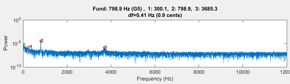
The analysis found two modes – the first was at 798.9 Hz and the second was at 3685.3 Hz. (It also found a little false mode at 300.1. bit that is just an artifact of the analysis and should be ignored). The target frequency for this F4 bar was 350.8 Hz, so I had a long way to go to get it tuned.
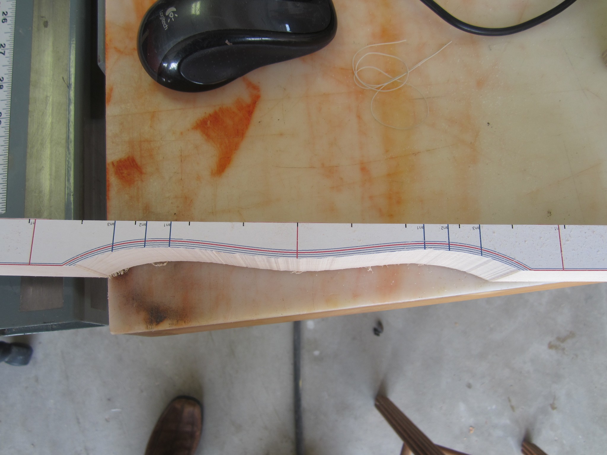
Next, I cut out the profile on the band-saw, as shown in the following photo.
(For those of you wanting to see more photos and explanation of the woodworking mechanics, please stand by. I will sort of gloss this over in the next few posts and focus on the practical realities of the math, and will later post details on the woodworking mechanics).
It may be hard to tell from the photo, but I made the first cut 3 mm proud of the computed red line. My intention of cutting way proud of the computed curve was to build some intuition regarding the sensitivity of the bar modes to wood removal. After this first cut, Jack took the bar back to the tuning jig and measured the frequency modes. After that, I used a drum sander to sand down to the 2 mm proud line and again measured the modes. After repeating the sanding and measuring steps on the 1mm line, we started the final tuning. Here is a table of the cut depth and the corresponding fundamental frequency.
| Standoff (from red line) | Fund Freq |
|---|---|
| +3 mm | 798 Hz |
| +2 mm | 415 Hz |
| +1 mm | 374 Hz |
| +0.5 mm | 360 Hz |
This was looking encouraging; we were only about 0.5 mm proud of the computed red line, and we were only about 10 Hz sharp. At this point, we alternated between the sander and the tuning station in a effort to “walk in” to the desired. However, we could not reliably measure the frequency of the second partial. For example, here is a power spectral density (PSD) plot after we had taken a few shaves with the sander.
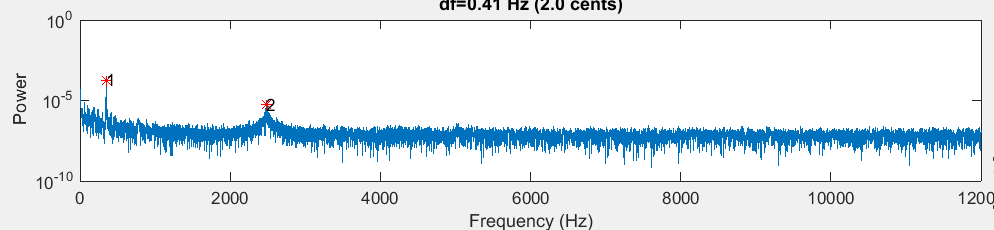
This data was collected by striking the bar at the center. There are strong first and third partials, but the second partial is not measurable. By accident, we hit the bar off the center – more toward one of the ends. Interestingly, we now measured energy in all three partials, as shown by the the next plot.
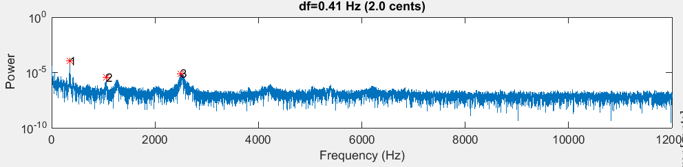
After discovering this, we routinely hit the bars off center to ring up energy in the second mode. (I found out later, after talking with some percussion professionals, that this knowledge is not wasted on xylophone players who are taught to hit the bar at a point that is just off center in order to yield the best timbre. However, I bet they don’t now why…)
Here were the resulting stats for this strike.
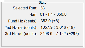
The is pretty good – the fundamental was at 352.0 Hz, which was just 6 cents sharp. The 2nd partial had a ratio of 3.016 and was 9 cents sharp. The 3rd partial, which we had decided we were not going to tune, happened in at a ration of 7.122.
Since the bar was still sharp, we continued sanding toward the profile. For this bar, the first and second partials were both sharp, so we removed wood mostly evenly across the full center portion of the bar. After a few more light sandings, we ended up with the following stats:
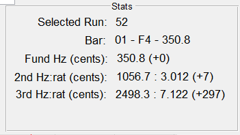
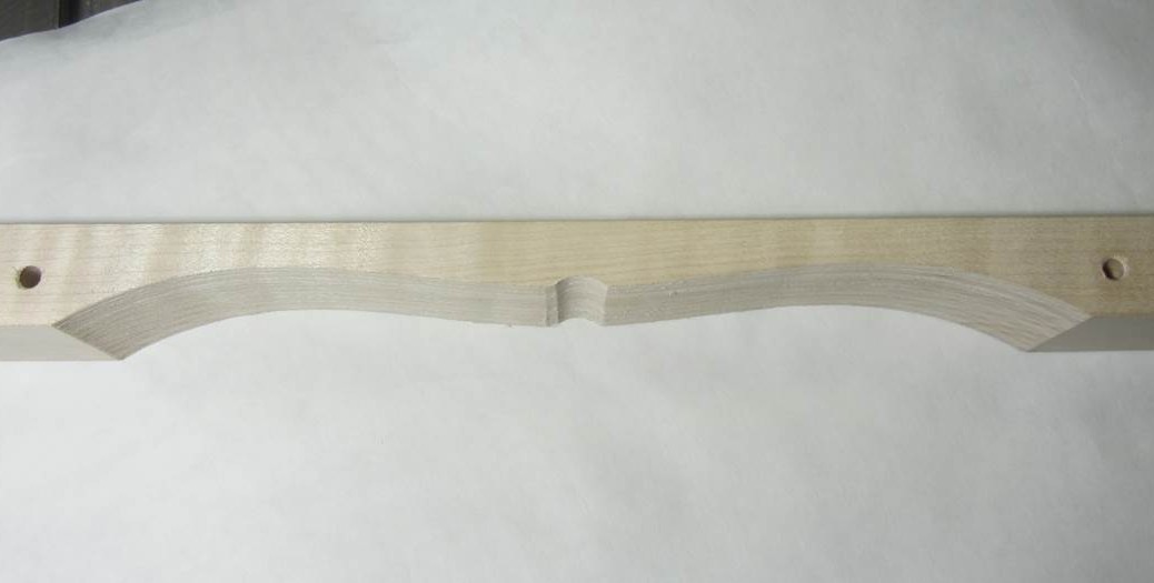
At this point, the fundamental was spot on, but the second harmonic was a bit sharp. Given the tuning curve above, there is really no way at this point to flatten the second mode without also flattening the fundamental. On the subsequent bars, I followed my tuning algorithm more carefully (i.e., bring the second partial into tune, or perhaps a tiny bit sharp, and then remove wood at the center to tune the fundamental) rather than just removing wood even with the fiducial lines. Here are a couple of photos of the final “tuned” bar.
It may be hard to tell from the picture, but the final cut is a small fraction of a mm above the computer prediction – I was pretty stoked! The math seemed to work!
Here’s a picture of Jack with our masterpiece: