Category Archives: Xylophone

A Bit More Math…

In the previous posts, I described the basic construction and tuning of a maple xylophone bar and promised that we would get into the woodworking next. However, we’ve got to do a bit more math first. Sorry for another bait-n-switch….

Rosewood Properties

As you may recall, the computer code that computes the bar shape requires the bulk modulus, shear modulus, and density to be specified. Apparently I am incapable of learning a lesson and again turned to the internet to provide these numbers. Like many of my previous attempts, I came up empty handed. Considering that all great Xylophones and Marimbas are made of one material – Honduras Rosewood – you might think that someone would have posted the material properties on the internet. If they did, Google and I couldn’t find it. This left me determined to compute them myself.

I did find a range of values for Young’s modulus (aka the bulk modulus) in a paper by Brémaud, et al. Figure 3a of the paper provided Young’s modulus values for  Honduras Rosewood (latin name Dalbergia Stevensonii) that span the range of 17-26 GPa. I am not sure why the range varied so much. Perhaps it is just natural variation in the wood? As an interesting aside, figure 3b of that same paper clearly shows that Honduras Rosewood has the lowest damping coefficient of all of the species evaluated, which the paper suggests is perhaps the most important quality for wood used to construct idiophones- this wood really is special.

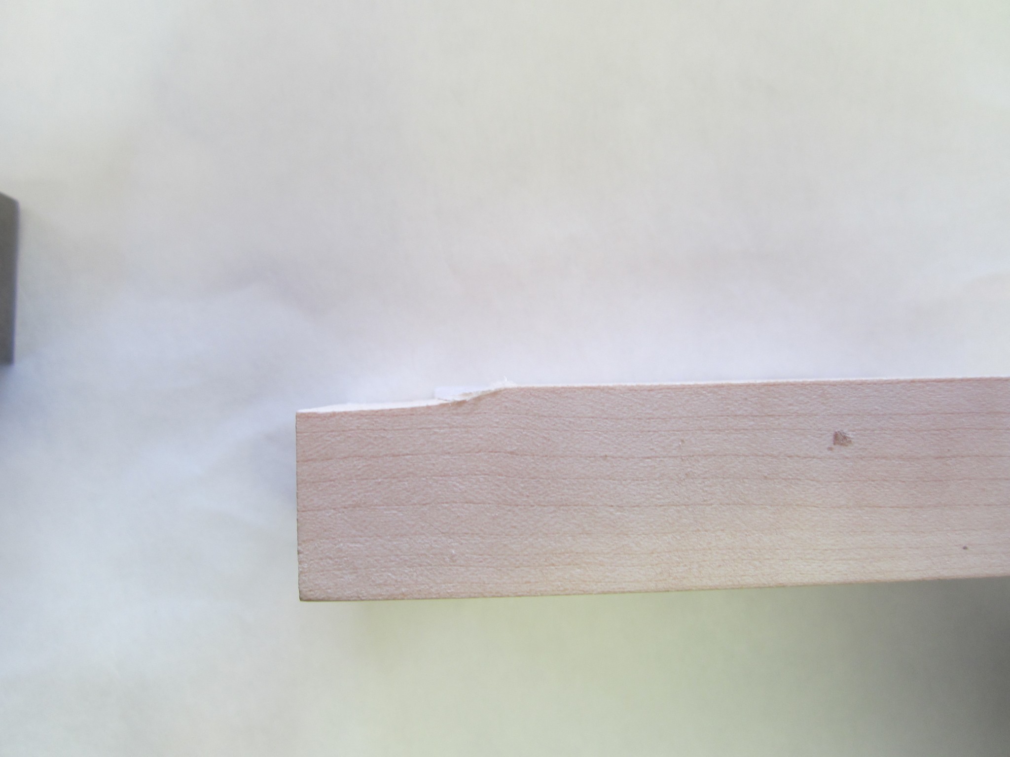
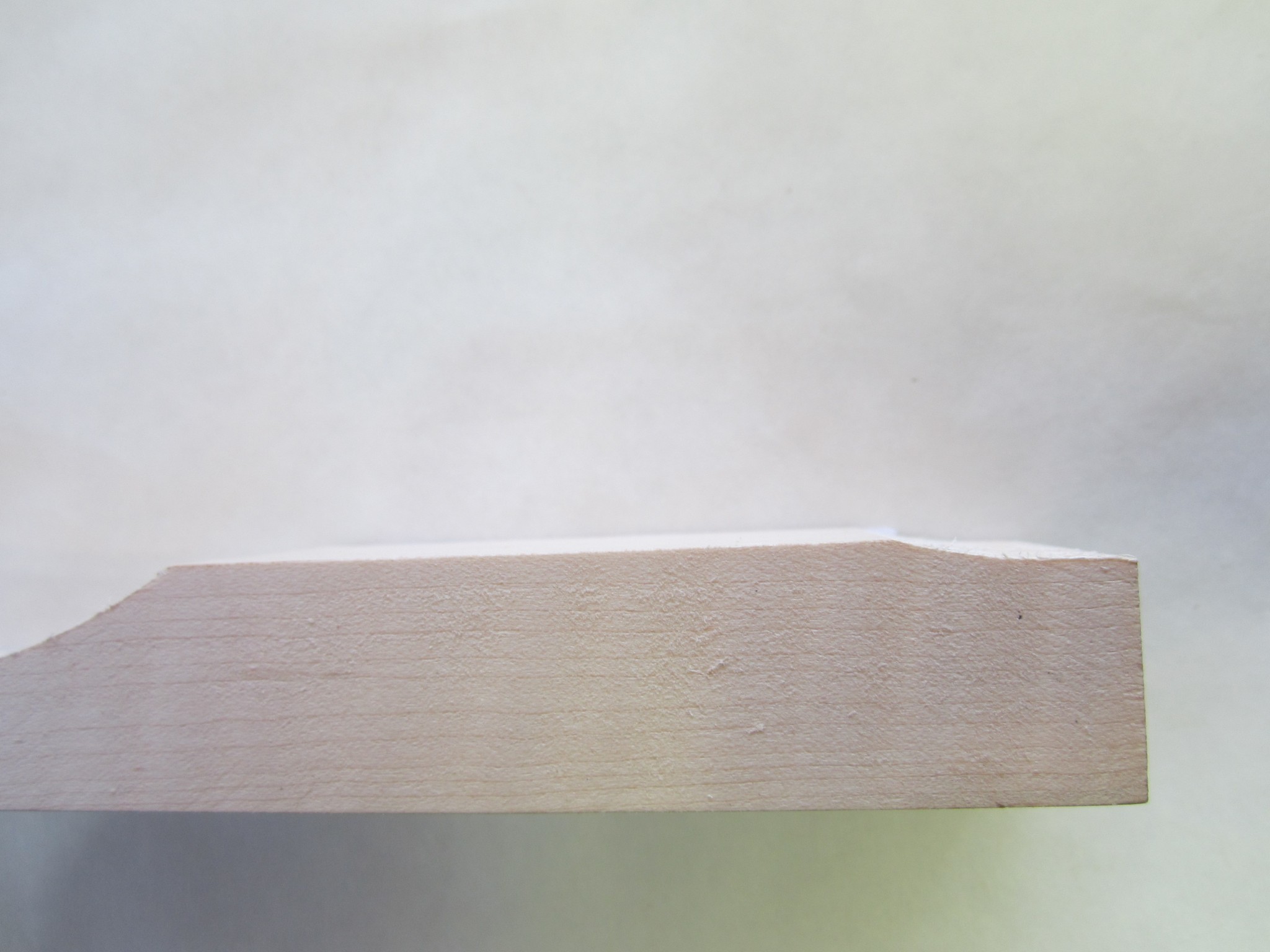
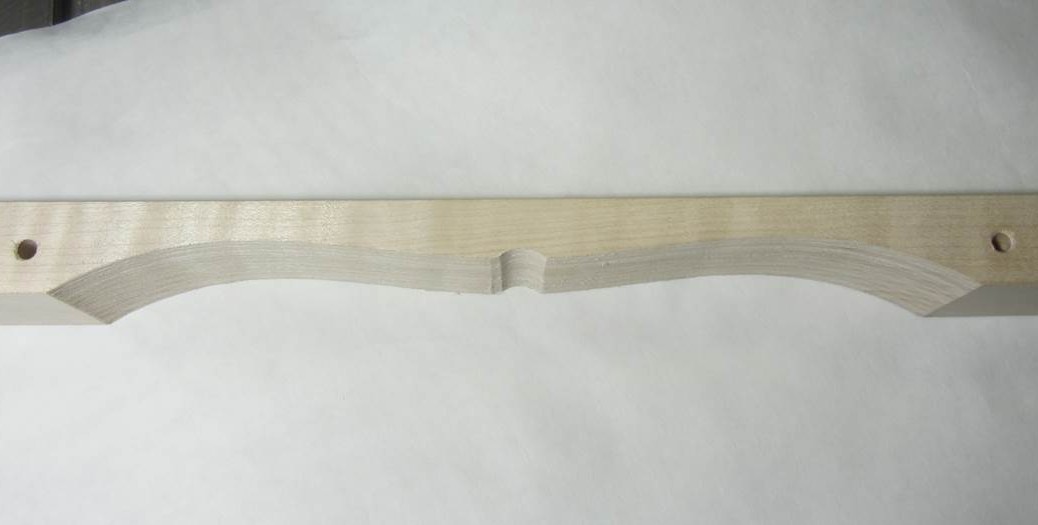
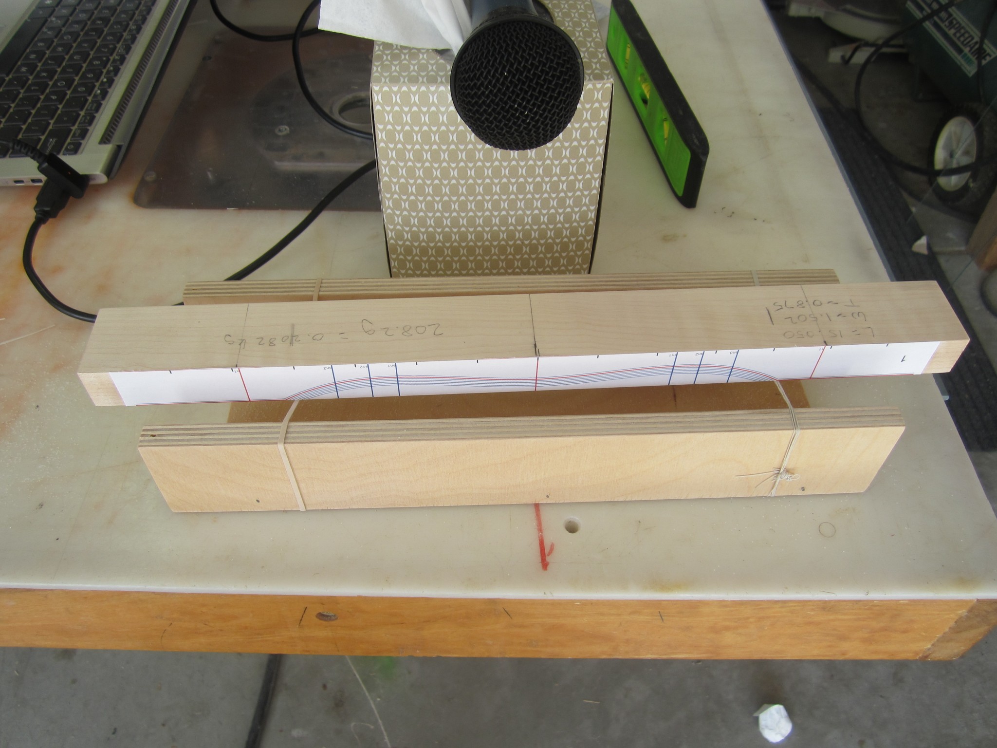
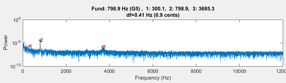
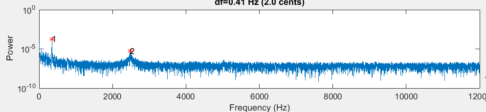
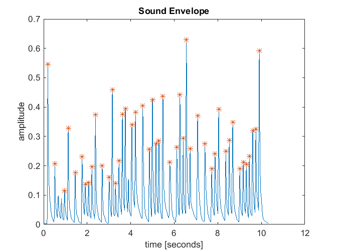
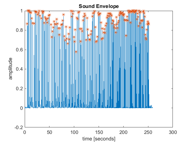
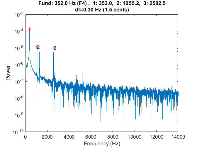
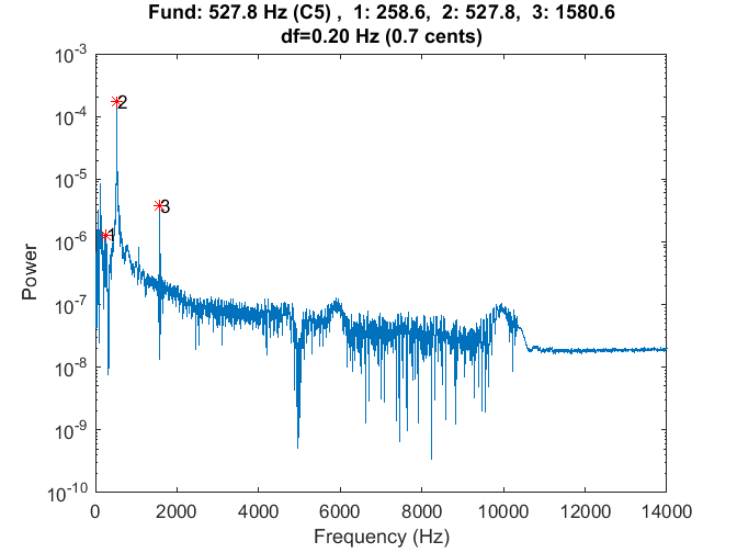
But the Zhao paper (and a few others that I found) came to the rescue. Appendix B of that paper, “Calculations for the Mechanical Properties,” provided a formula for calculating Young’s modulus from the fundamental frequency of a prismatic beam constructed from the material. My first job was to whack a Rosewood bar of known dimension and measure its fundamental. I had a couple of rosewood “test bars” that I cut to mess around with, and the longest one was 13-5/64 inches long. Here is the spectrum of that bar.

Spectrum of my longest rosewood test bar.
Spectrum of my longest rosewood test bar

And here is the sound file for your listening pleasure.

From the spectrum, you can see that the fundamental was at about 957 Hz. You can check out the Zhao paper for the details of the equation, but here is the Matlab code to compute the modulus. (Note that the Zhao paper had an error in equation for E where beta_n should have been the constant beta_n*l)

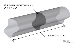
inch2m=0.0254; %Conversion constant

%Compute the young's modulus from bar #1
b=1.501*inch2m; %width
h=0.880*inch2m; %height
L=(13+15/64)*inch2m; %Length

f1=957; %Measured frequency of fundamental
rho = 1082; %Density from measurement of volume and mass (see above)

A=b*h; %Cross sectional area
I=b*h^3/12; %Moment of inertial

E=4*pi^2*rho*A*L^4/I * (f1^2/4.73^4) %4.73 is a constant given by Zhao
%E = 2.396974370897572e+10

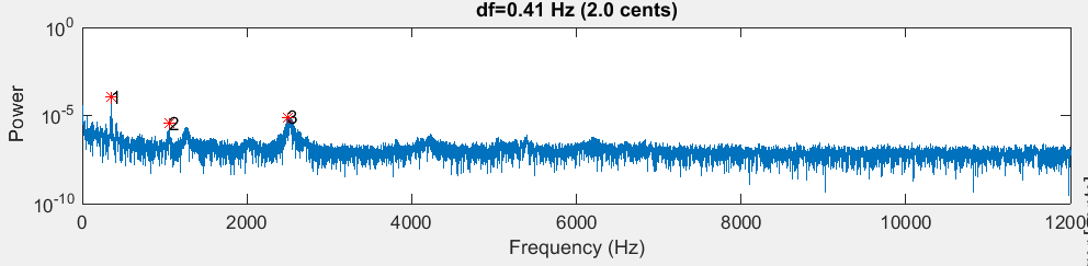
The modulus calculated for this bar was 23.9 GPa. I had a second bar that had a length of 9-27/64 inches and a fundamental frequency of 1867 Hz. The calculated modulus for this bar was 23.6 GPa – pretty close to the first number.

Zhao also gave a formula for the calculation of the shear modulus, G, but the torsional frequencies of the bar must be known. It was not clear to me that I could adequately “ring these up” and measure them, so getting the shear modulus using that approach seemed off the table. I decided to take a different tact.

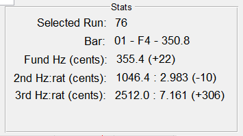
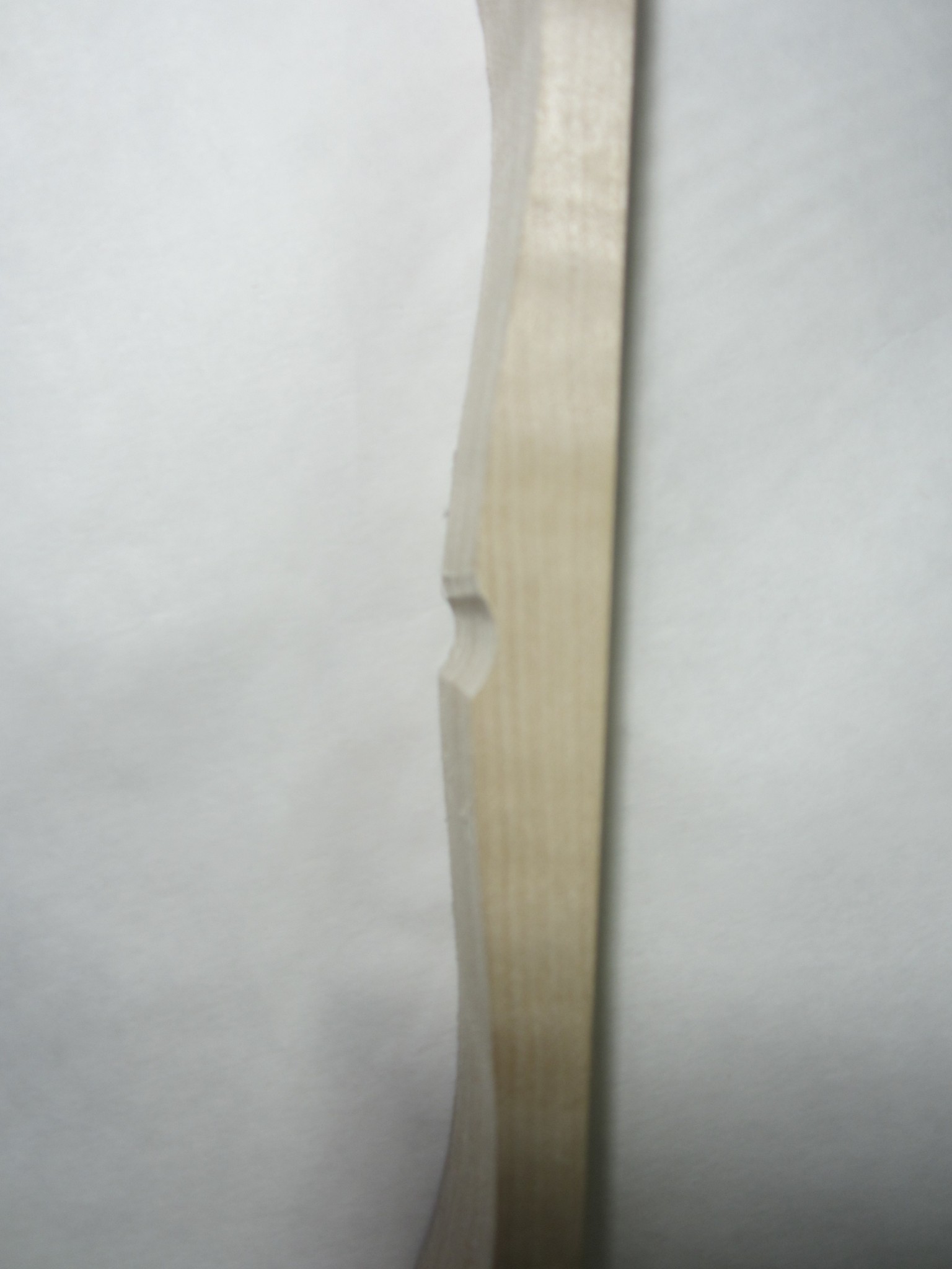
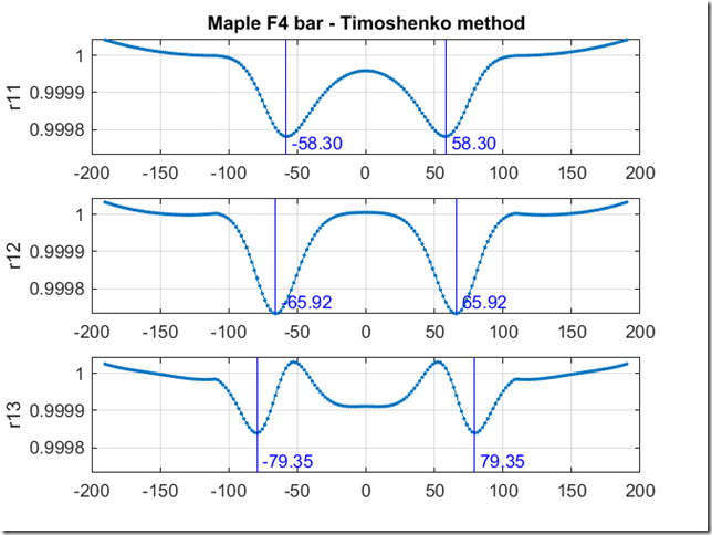
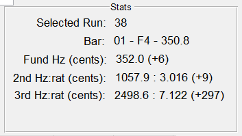
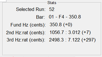
My approach was to do a parametric sweep of the shear modulus using the Timoshenko code to compute the fundamental and first two overtones for a prismatic beam. My idea was that if I had the bulk modulus and density right (density was easy, I just weighed and measured the bar and divided the numbers,) then the only free variable was shear modulus. If I adjusted it until I made the Timoshenko-predicted frequencies match the measured frequencies, then I must have the right value for the shear modulus; right? Here are the results from that sweep for the long and short test bars.

Shear modulus sweep for my long test bar.
Shear modulus sweep for my short test bar.
Shear modulus sweep for my short test bar

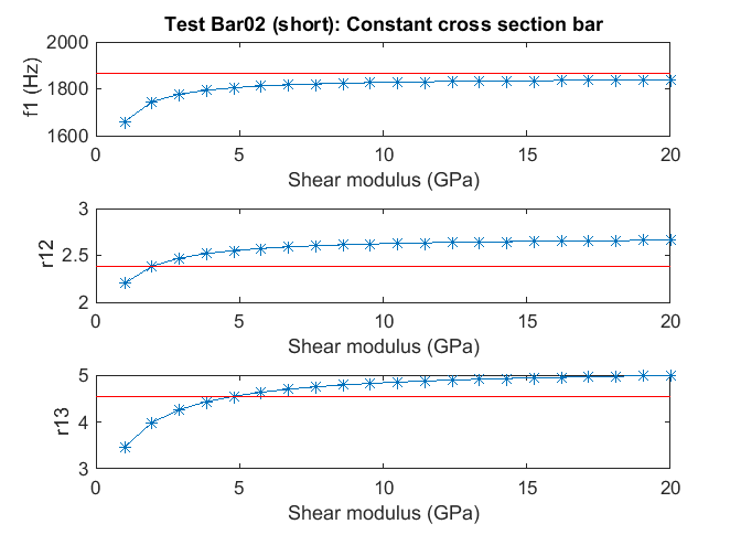
The red lines on the plots correspond to the measure modal frequencies based on my spectral measurements. This analysis was not entirely satisfying because the no value of G yielded the fundamental frequency – the prediction was always a bit lower than the measured value- however, inspection of the second and third partials suggested that a reasonable value for the shear modulus might be around 4 GPa.

For what it’s worth, I did find a published shear modulus value of 19 GPa for Padauk, a similar wood. This suggests my chosen value of 4 GPa might be too low, but I wasn’t sure what else to do – high values resulted in a very poor match for the overtones in the plots above. For what it’s worth, I computed some bar profiles with different values of G, and they didn’t vary a lot. So perhaps at the end of the day it’s not a big deal, since I knew I was going to have to “hand tune” the bars after roughly cutting to the computed shape anyway. Right or wrong, I forged on with my value of G=4 GPa.

Summary of Computed Results

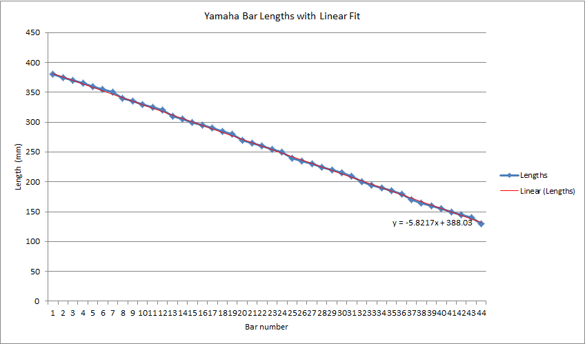
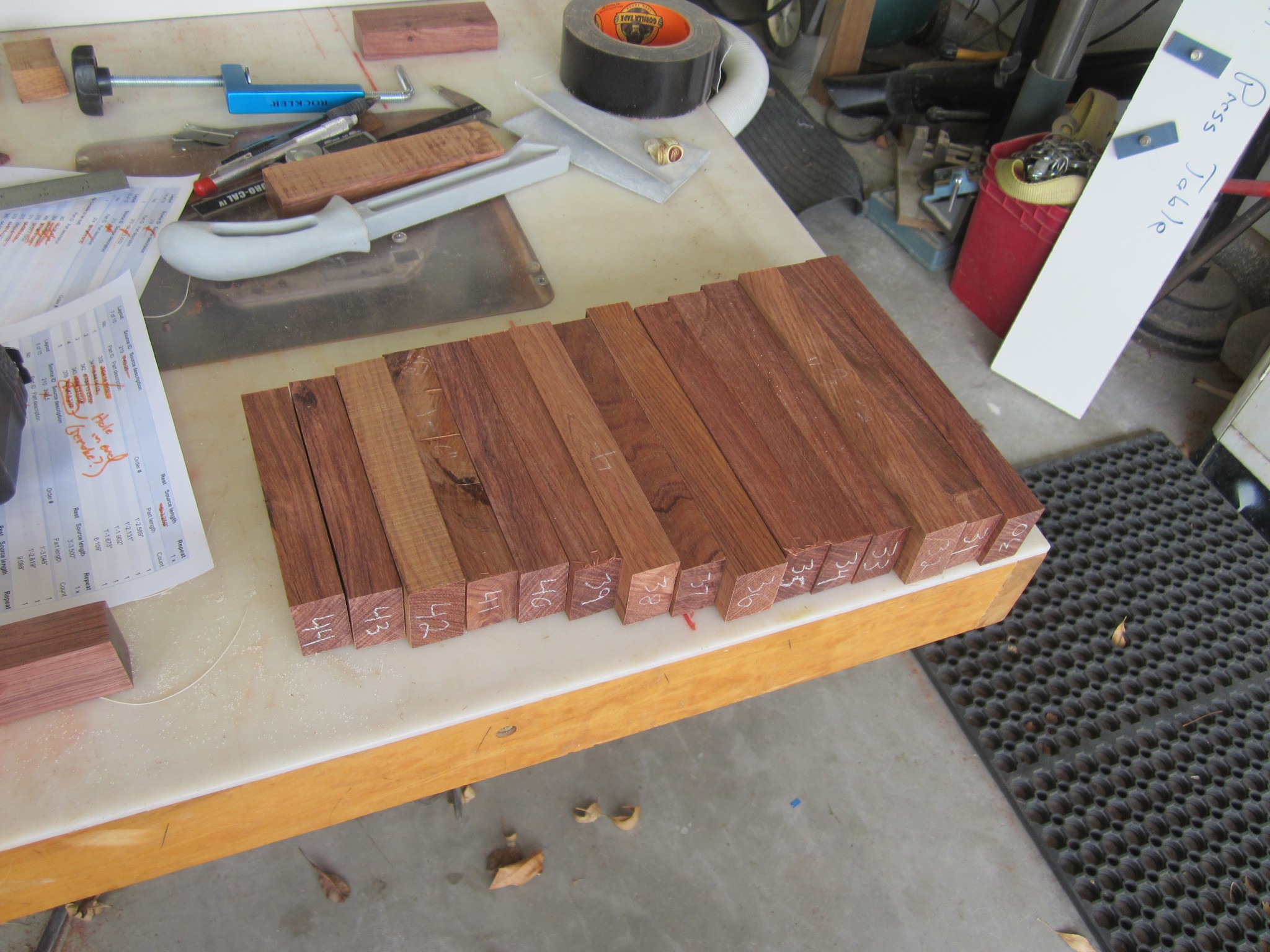
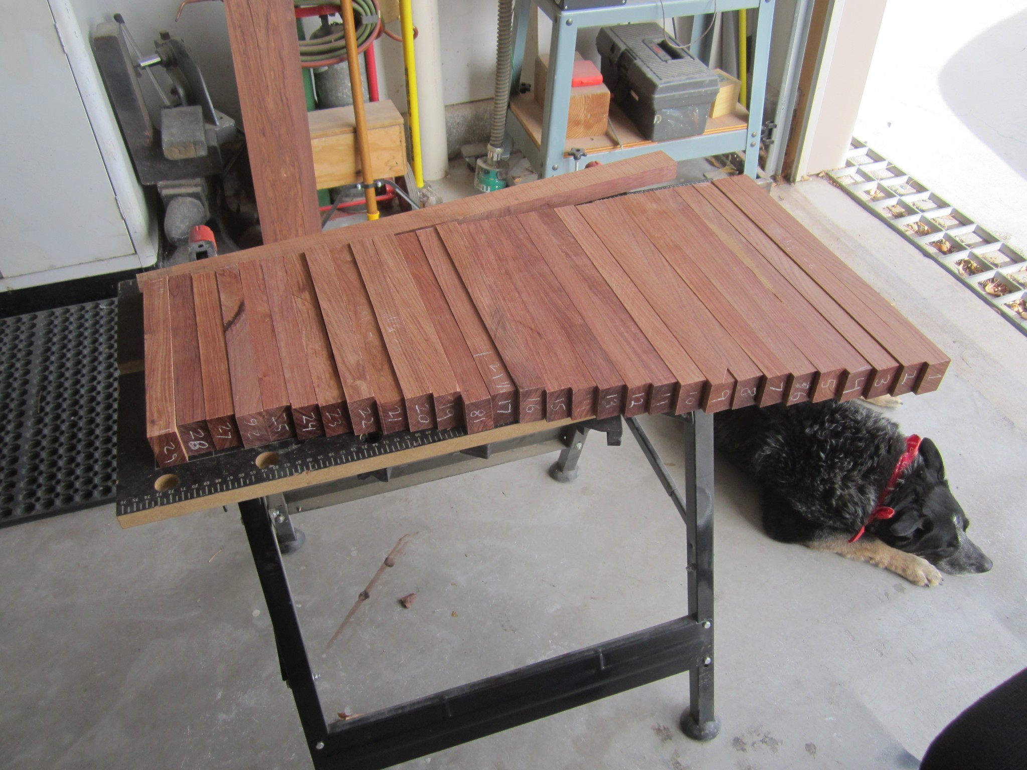
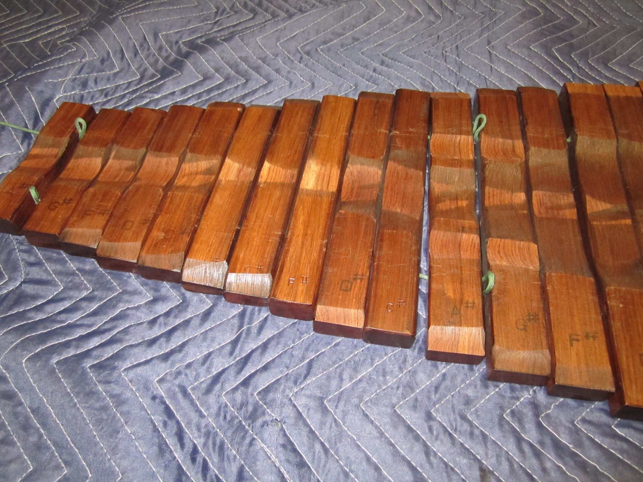
With the Rosewood material properties estimated, I was able to run the minimizer/Timoshenko code to compute the bar profiles for each of my 44 rosewood bars. As I mentioned in a previous post, the minimizer is sensitive to the initial starting condition, so I seeded my first and longest bar, F4, with the cubic coefficients from the maple bar and watched the minimizer converge. For the rest of the bars, I initialized the minimizer by seeding it with the coefficients from the previous bar, working my way from longest to shortest. In this manor, I was able to leap-frog through the bars and ensure that the minimizer converged.

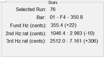
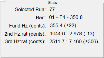
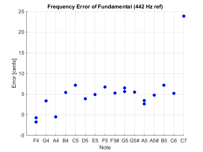
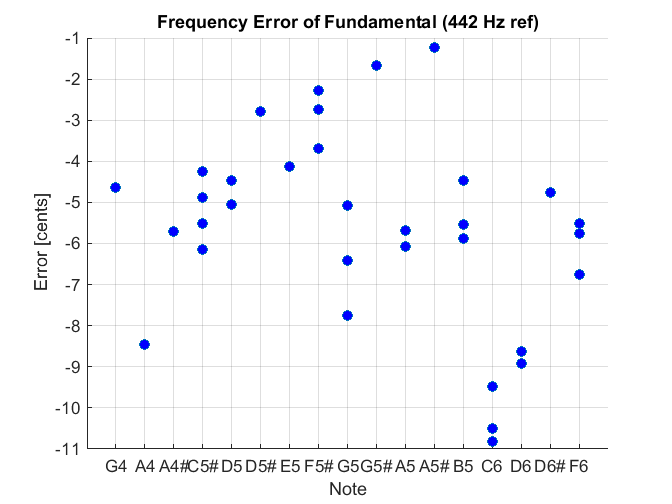
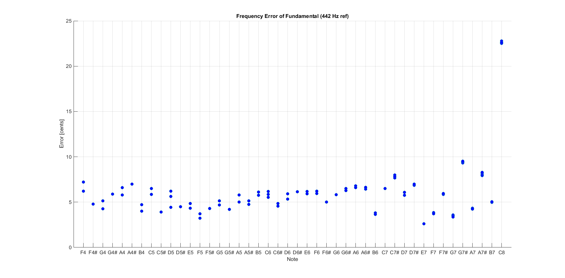
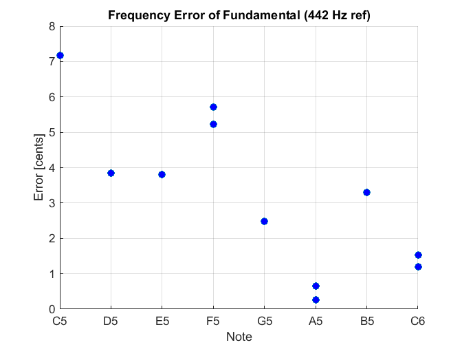
Here are some summary results from the computed bar runs. First, here are the fundamental frequencies as calculated by the Timoshenko and Euler methods for each of the bars.

Computed fundamental frequency for all bars via two different methods.
Computed fundamental frequency for all bars via two different methods

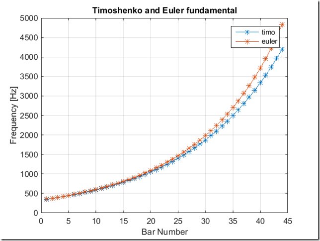
In every case, the code was able to perfectly converge to the desired fundamental frequency. The plot shows the results for the two methods. As previously noted, the Timoshenko method is generally more accurate, especially for the short bars.

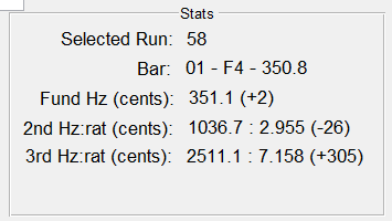
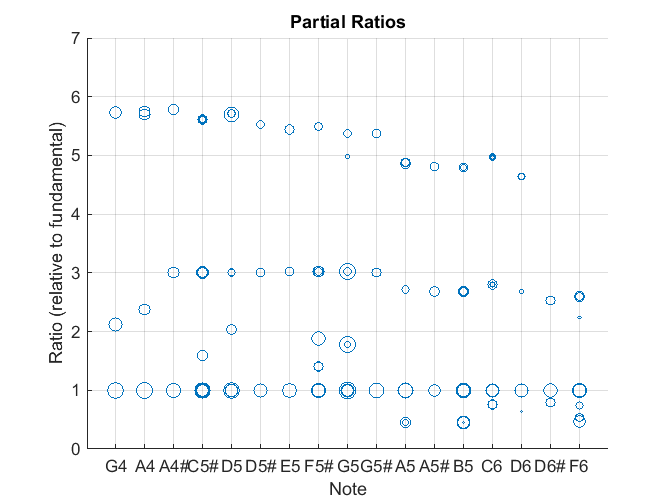
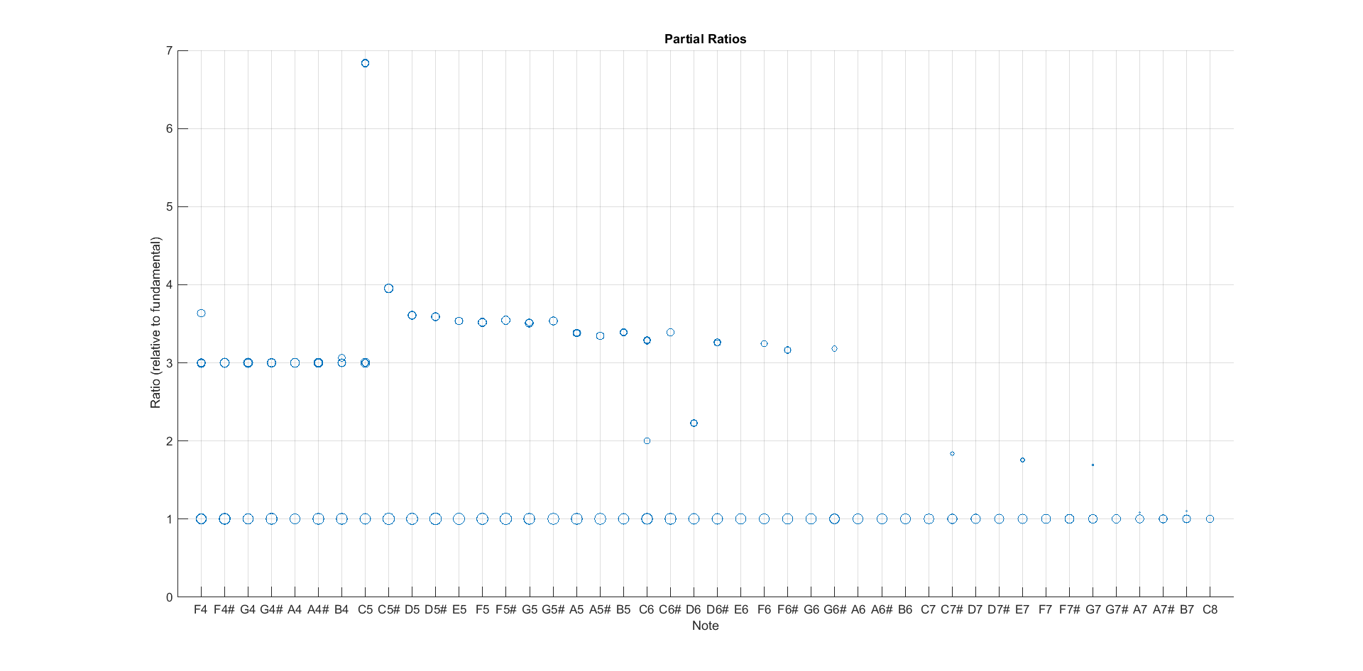
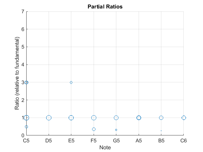
Here are the ratios for the second and third overtones:

Computed ratios for the first two overtones.
Computed ratios for the first two overtones

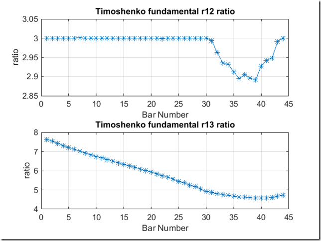
I found it interesting that the code can’t converge on the 2nd overtone for the short bars. No big deal because the overtones decay so rapidly for the shorter bars, it is doubtful that this effect can be heard. Indeed, when I was tuning the shorter bars, my spectral measurements were not able to measure the overtones.

The Templates Please

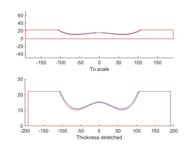
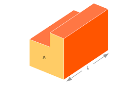
The computer run for each bar produces three standard plots. The first is the bar profile plot. An example for bar 10 is shown here.

Profile plot for bar #10

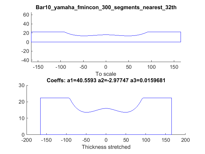
You’ve see plots like this before. The top figure has a 1:1 aspect ratio and gives an idea of the actual physical profile of the bar. The bottom figure has a arbitrary aspect ratio to better visualize the shape of the undercut. Also included on the figure are the coefficients for the cubic function that describes the profile curve. I followed Dr Entwistle’s definition for the cubic coefficients where

y=a1*x^3 + a2*x^2 + a3;

In this equation, x is the longitudinal length down the bar where x=0 is the bar center. The variable y denotes the bar thickness corresponding to each value of x. Notice that when x=0, the equation reduces to y=a3, which is the thickness at the center. Also, notice that there is no linear term with x (i.e., no coefficient that multiples x). Setting the linear coefficient to zero forces the cubic function to have zero a slope at x=0. This forces symmetry about the bar middle.

Note that there is nothing magical about using a cubic to represent the bar shape. Indeed, if I were going to build another xylophone, I might mess around with other functional forms to see if I could satisfy additional constraints, like forcing the third partial ratio to be 6.0, or to maximize sustain or volume. However, the cubic is a good compromise in that does a respectable job of providing shapes that mimic what I had seen on other xylophones while keeping the degrees of freedom low (i.e., just 3 coefficients).

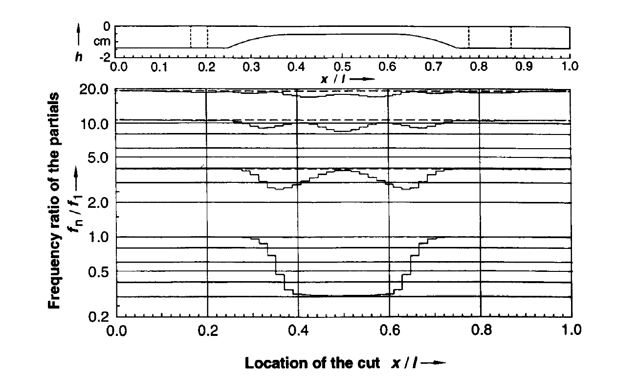
The second standard plot that I compute is the tuning curve, which we have discussed at length. For completeness, here is the tuning curve for my #10 bar.

Tuning curve for bar #10

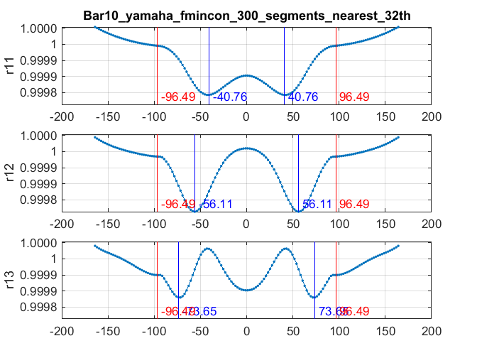
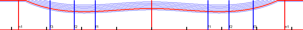
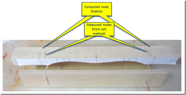
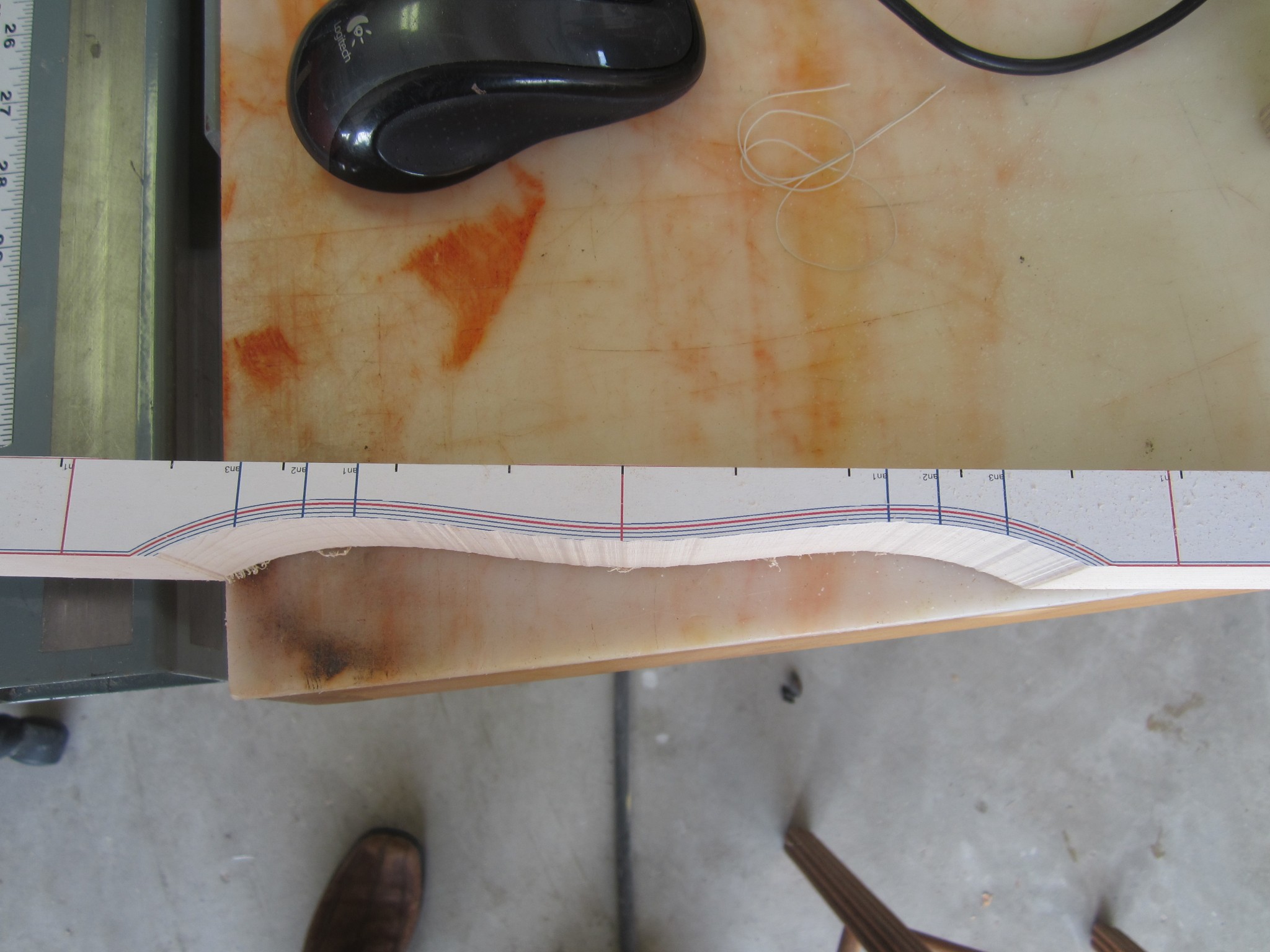
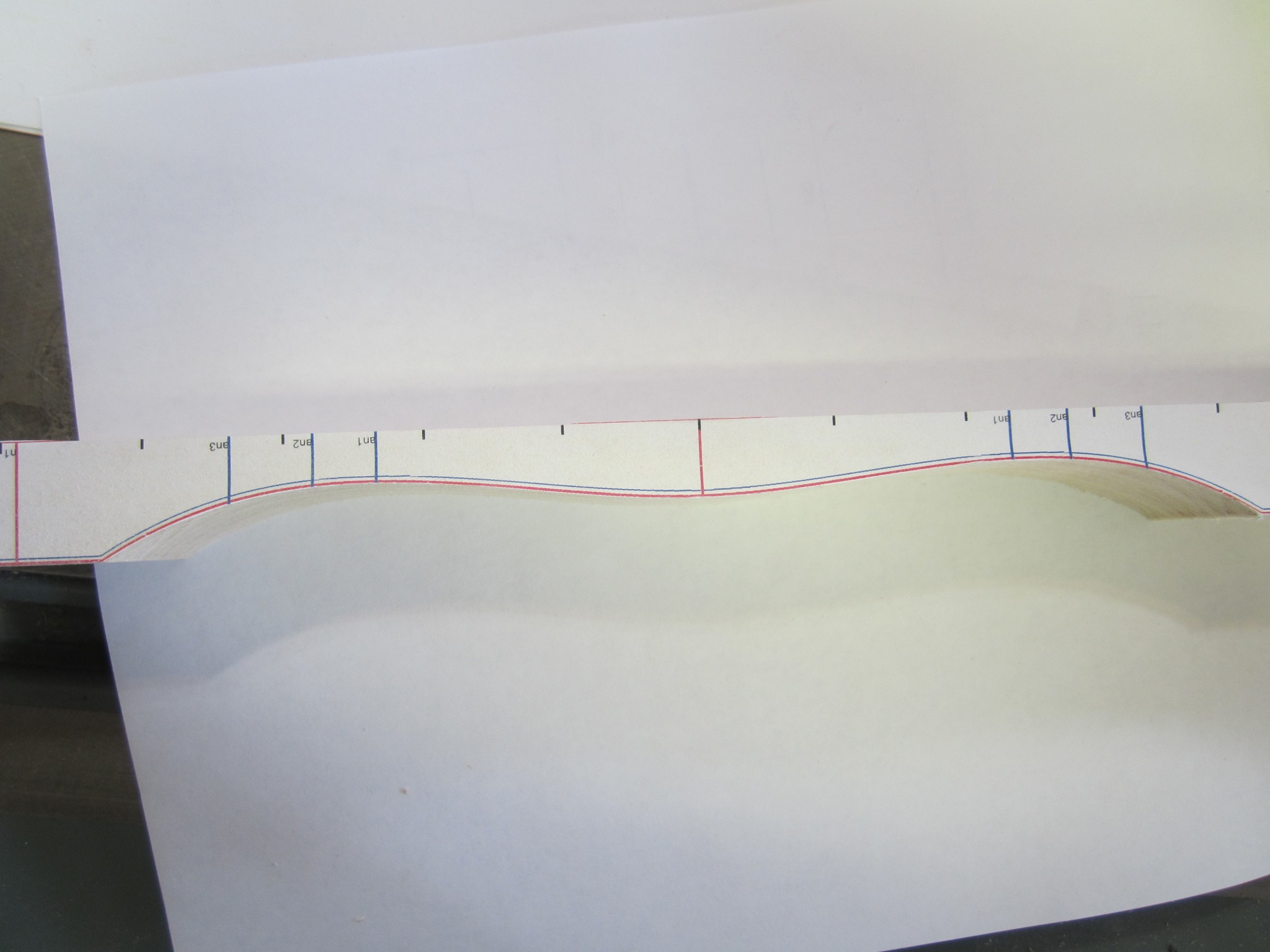
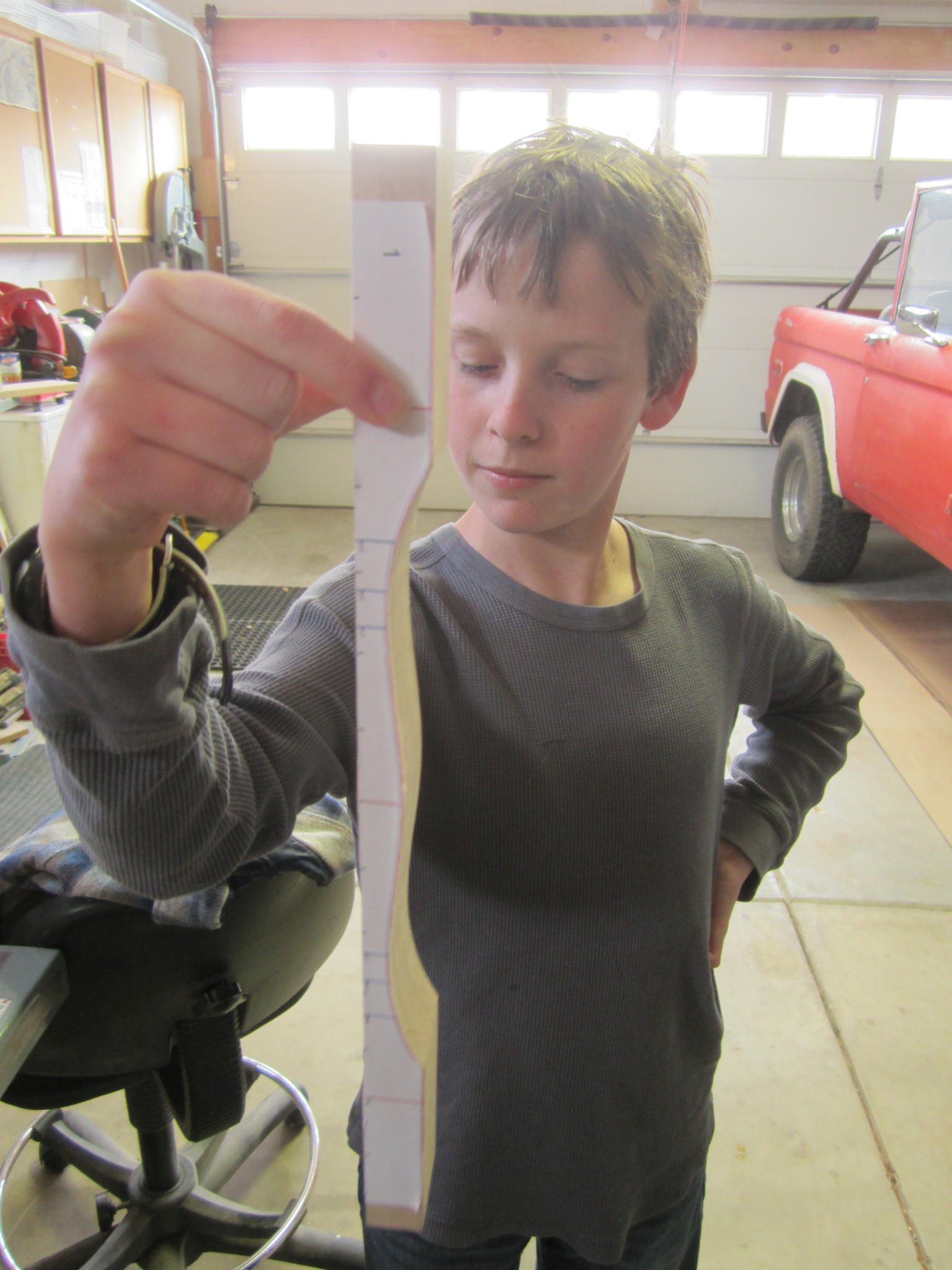
Finally, as described in the maple bar fabrication discussion, I create a full-size paper template for each bar. Here is the template for bar #10:

Template for bar #10

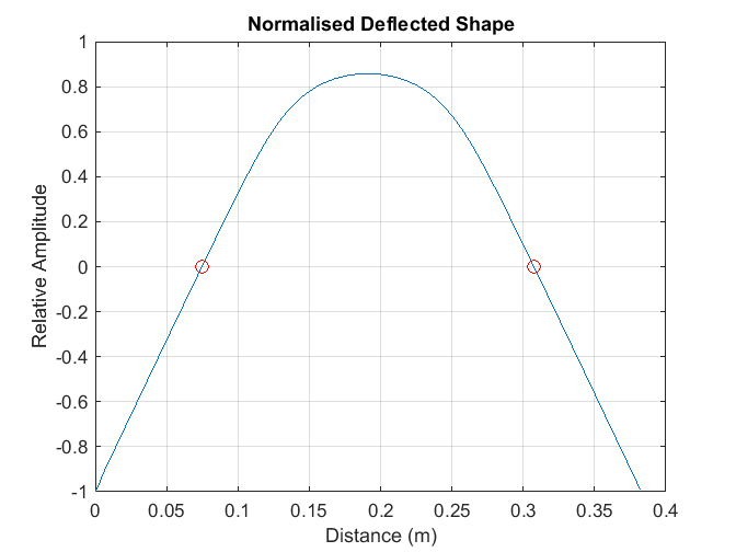
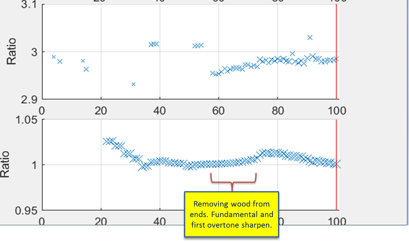
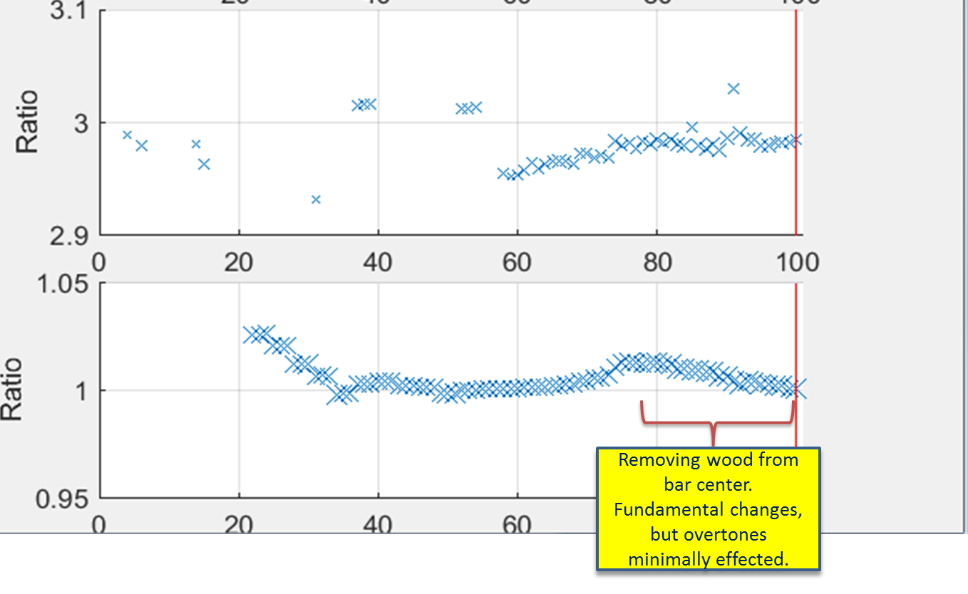
A couple of notes about the annotations on this template are in order. The two vertical red lines mark the node locations as computed by the Euler code provided by Dr Entwistle. These are where the holes will be drilled. The vertical blue lines, marked f1, f2 and f3 denote fiducials on the bar corresponding to the tuning curve peaks. The f1 mark denotes the location where the fundamental is most affected by wood removal. Similarly, f2 marks the location where wood removal most dramatically changes the second partial, and f3 corresponds to the most sensitive region for the third partial.

All of these are useful plots, so I have zipped up the three curves for each of the 44 bars into a single file for you to download…I am just that kind of a guy 🙂

Here is the zip file: standard_plots_for_all_44_bars

Note that each of the files is a PDF, including the bar templates. The templates’ PDF files have been created so that they should print full-size. I made these to print on 8.5 x 14 inch paper, which was the largest size that my printer would handle. I am not sure how they will print on a smaller page size, but in any case, you should be able to scale these based on the bar sizes that I provided in the Excel file in the previous post.

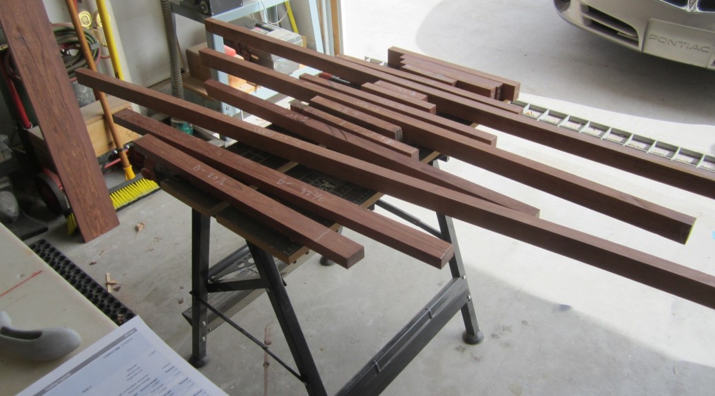
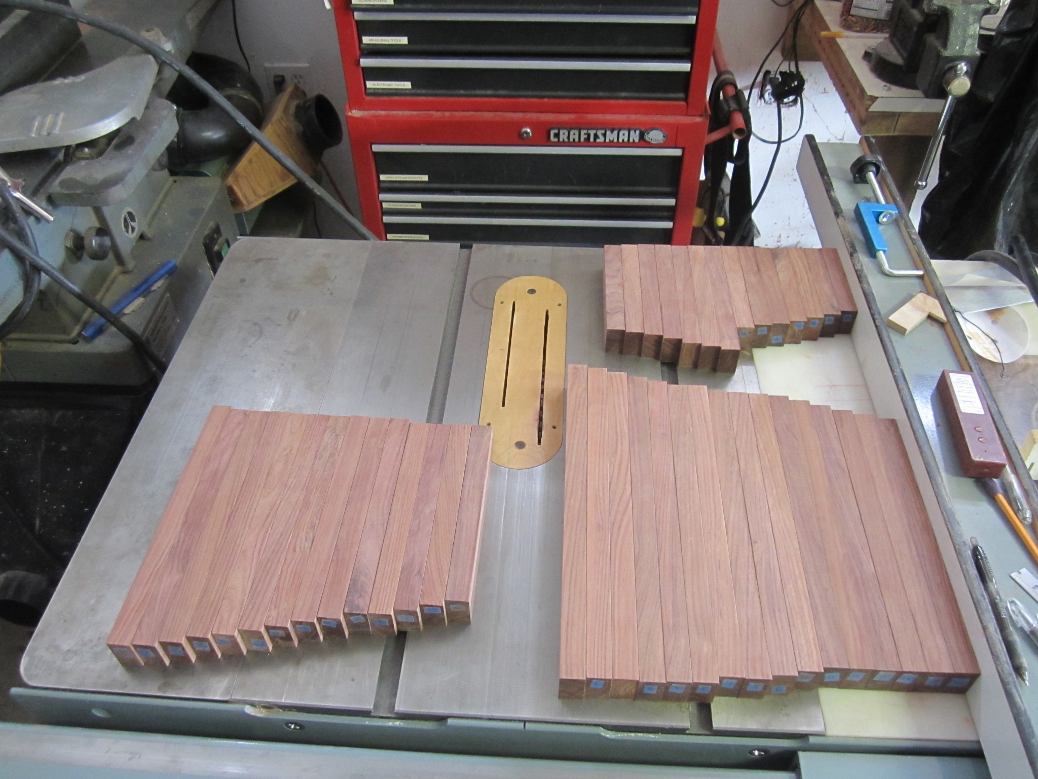
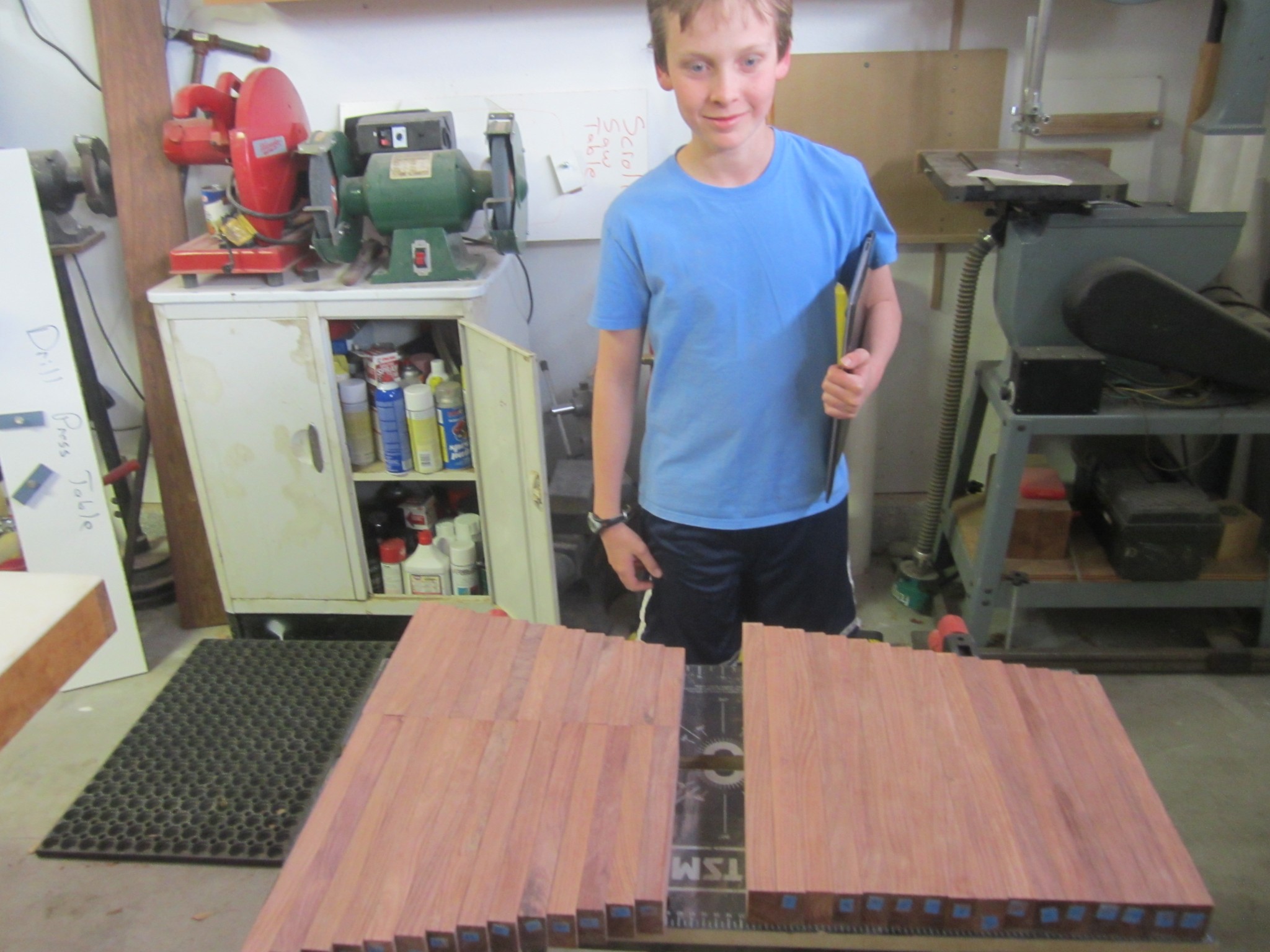
In the next post we will actually start cutting Rosewood. (I know, you’ve heard that before. But you didn’t think you could build a xylophone without math, did you?)


References

Iris Brémaud, Pierre Cabrolier, Kazuya Minato, Jean Gérard, Bernard Thibaut. Vibrational properties of tropical woods with historical uses in musical instruments. Joseph Gril.International Conference of COST Action IE0601 Wood Science for the Preservation of Cultural Heritage, Nov 2008, Braga, Portugal. pp.17-23, 2010. <hal-00808403>


Rosewood

With our newfound knowledge of tuning xylophone bars, Jack and I were prepared to go all in – time to buy the rosewood.

We live in Albuquerque, which is not a large city, so I was prepared for a protracted search for affordable rosewood. I found a few sites online, but all were pretty spendy and mostly catered to users buying small quantities. On a whim, I checked out a local vendor called Albuquerque Exotic Hardwoods (now called World of Wood). To my surprise, they had just received a small shipment of Honduras rosewood! The owner explained that there were some “quality issues” so they were selling it for half price.

Like most woodworkers, I typically seek out stock that has the most interesting grain. I generally build furniture that has simple lines and let figure in the wood provide the interest. In selecting stock for this project, I had to fight that urge and select the most boring planks, since these will typically be the most homogeneous. This nearly killed me, and to own the truth, I bought one extra plank that was highly figured and just too pretty to leave at the store.

I know you are going to ask what the price was, and I’ve racked my brain trying to remember, but I’m afraid those brains cells got displaced by bar tuning math. I can tell you that I spent about $200 total on the rosewood. As noted, the wood had some checks and knots that I had to cut around, so I estimate that had about 30% waste. (But did I mention that the wood was half price?!)

The width of the bars doesn’t greatly affect the timbre, so I sized them to be consistent with what I had nominally observed on commercial xylophones. The Yamaha that provided my sizing template had bar width at 1.5 inches, which was right in line with most other xylophones I had seen. The rosewood boards that I bought were mostly about 5-7 inches wide, so for each board I figured out how many widths I could rip out of each plank and started cutting.

When I began ripping these on my table saw, I got my first surprise; despite selecting boards with pretty straight grain, there was so much internal stress in this wood that after ripping the first six inches or so, the piece against the table saw fence (the 1.5 inch strip I was ripping off) started bending badly against the main plank. This is not uncommon when rippling hardwood, but I’ve never seen it this extreme. It is also a serious problem, because as the wood bends out it tends to push laterally against the blade, causing binding and burning. It can also result in pieces that are thinner than the 1.5 inch width target. Not every cut had this problem, but probably half of them did. I am not sure if this is a common problem with rosewood, but I definitely had to address this challenge. So I did two things. First, I ripped the pieces about 1/8 inch wider than the necessary final dimension to allow for thinning that resulted from the bending board.

My second mitigation was to put a screw in the end so the ripped piece couldn’t bend out too far. I wish I had a photo of this, but I didn’t take one, so here is a cheesy illustration that will hopefully make clear how I addressed this issue.

Screw used to capture bending ripping piece.
Screw used to capture bending ripping piece

Basically, I would rip the board about 8 inches and them drill a pilot hole at a 45 degree angle. Then, I would drive a wood screw to straighten the 1.5 inch part and pull it back toward the main plank. After this, I would restart the rip, but of course I couldn’t cut through the screw, so rather I would plunge the blade into the existing cut past the screw, then finish the rip cut. This process slowed down the ripping tremendously, but it did tame the board so that I could get decent (not great) cuts. Of course, the resulting ripped boards had a gnarly curve to them, but recall that they only needed to straight over the length of the bar (less than 15 inches).

Once I used this technique to rip all of the pieces, I cut out all of the bad chunks. This included knots, splits and checks. This left me with a number of boards that were various lengths, so now I was ready to rough-cut all of my bars from these stock pieces. You can see some of the ripped pieces at the post at the top of this page.

Optimizing Board Usage

With my boards ripped, the next step was to determine the exact lengths for my 44 bars. Recall from a previous post that I chose to use the lengths from a Yamaha instrument I found online. I entered all of the bar lengths from the Yamaha parts list and created the following plot.

Yamaha bar lengths
Yamaha bar lengths

There is a bit of wiggle in the points due to rounding in the published Yamaha data, so I added a linear trend line to average out the “noise,” and used that to compute the lengths for each bar. The bar lengths are contained in this Excel file: bar_lengths

At this point, I had my stock ripped to 1.5 inches, and I had exact lengths for each of my 44 bars. Now many times over the years I have ran into the problem of efficiently cutting a number of lineal pieces from a set of stock material lengths. The classic example of this is cutting baseboard molding where you buy nominally 12 foot boards and chop them up according to your wall lengths. In general, the problem can be solved by trial and error – basically guessing at how to best divvy up the needed pieces into the available stock. However, because the rosewood is just a bit more expensive than baseboard molding (pause here to let the point sink in,) I attempted to be as efficient as possible.

I turned back to the internet to see if I could find some software to help. There were a couple of free programs that I found, but they were pretty cheesy and difficult to use. Ultimately, I ended up downloading a trial version of a program called Cutlist Plus. This software is pretty sweet in that it lets you enter all of your stock lengths and the desired finish pieces, and then computes the optimal assignment of pieces to stock. The program takes some getting used to, but it is very flexible and produces very detailed printouts that make it easy to stay organized. I seem to recall that the trial version is good for month. They have a $39 version aimed at hobbyists, but it only cuts sheet goods (i.e., two dimensional pieces like plywood,) not lineal pieces. The full version is $250, which was too rich for my blood. (Please let me know if anyone out there knows of inexpensive software that performs this function – it would be nice to have it around for occasional use).

After rough-cutting all of the pieces according to Cutlist Plus assignments, I dimensioned each bar to it final size. This included straightening on the jointer and ripping to final width on the table saw. Because I cut each bar a bit long, the final step was to cut each  to its finished dimension. The Excel file above contains a column with the lengths rounded to the nearest 1/32th of an inch. I find that my table saw rule guide is the most accurate and fastest way to cut short pieces like this, and the fractional column in the spreadsheet allowed me to quickly set the length.

As your reward for staying with us this long, here are some photos of our cut pieces!

Rough-cut pieces.
Rough-cut pieces
Rough-cut pieces.
Rough-cut pieces
Final, dimensioned pieces.
Final, dimensioned pieces
Jack checking out his handiwork!

In the next post, we will show you more of the woodworking steps involved with turning these “blanks” into tuned xylophone bars and a few challenges we encountered along the way.

Making a Friend

I wasn’t done torturing my maple test bar. As previously mentioned, xylophone bars are suspended by strings that pass through holes drilled at the nodal locations. From a practical standpoint, I needed to assess whether drilling the holes would affect the modes. If so, I would have to first “rough tune” the bar, drill the holes, and then finish tuning the bar.

Finding the Nodal Locations With the “Salt Method”

A few sites online, including the La Favre site, suggested using the “salt method” to determining the nodal locations.  This technique has you sprinkle salt on the bar in a random pattern, and then repeatedly strike the bar. Because the bar vibrates minimally at the nodal locations, the salt slowly migrates to the nodes. It’s really cool and sort of magical to watch. I didn’t take photos of the salt method applied to my maple bar, but here are some before-and-after photos of the salt migration for one of the rosewood bars.

Salt randomly sprinkled.
Salt randomly sprinkled
After salt had migrated to the nodal locations

The salt makes pretty clean little lines, clearly marking the location of the nodes. (As a brief aside, the lines are rarely perpendicular to the long axis of the bar – they are almost always angled. This is just due to the wood grain, which the MEs would refer to as “the non-isotropic nature of the material.”)

Jack and I used the salt method to determine the locations of the nodes for our maple bar and drew lines with a pencil though the middle of the salt lines. However, the results were surprising – the nodal locations determined by the salt method did not align with the “n1” locations predicted by the the tuning curves (refer back to the figure containing the bar template).

Recall that my n1 marks correspond to the location where the tuning curve crossed zero; that is, removing wood here has no effect on the modal frequency. I speculated that these zero-crossing points might be coincident with the nodal locations, reasoning that since wood removed here does not affect the fundamental, it might also identify the nodal locations. However, as noted above, that was not the case. Here is a photo with annotations showing the difference between the predicted and measured nodal locations.

Nodal location mystery.

The measured and computed node locations differed by about 1 cm. This disturbed me, because up until this point, all of the computer predictions had been spot on.

Making a Friend

So I went back to literature to see if I could find some clues. The Zhao paper that provided the original version of the beam software referred to a function called Drilled_Hole_Predictions.m.  A comment in the code indicated that this function would calculate the necessary location of the holes. However, the source code for this particular function was excluded from the appendix of the Zhao paper. As I have previously mentioned, comments in the source code indicate that it was derived by code written by Dr. Rodney Entwistle of Curtin University of Technology in Perth, Australia.

So I sent Dr. Entwistle a note explaining the mission that Jack and I were on and asked if I might trouble him to provide the missing function. To my great surprise, Dr Entwistle replied quickly and was very interested in our project! Being an amateur woodworker himself, and a father to four boys, I think he identified with the challenge that Jack and I had undertaken. So “Rod” and I begin a long series of correspondence that provided not only the node location function, but countless invaluable insights and pointers. Most importantly, his enthusiasm and continual encouragement kept me motivated to finish this project, even when it got tedius. Indeed, much of the material in this blog is the result of insights provided by Rod. I feel very lucky indeed to have found not just an expert who was willing to aid our pursuit, but a like-minded engineer that was a “geeked out” as I was by this engineering journey!

Back to the node location mystery. Rod pointed out that the nodal locations are not coincident with the zero-crossing computed by the tuning curves, and provided a function that computes the deflected shape of a beam. This code essentially computes the magnitude of deflection as a function of the longitudinal beam location. I used Rod’s code to compute the deflected shape curve for my maple bar, as shown in the following figure.

Deflected shape curve for the maple bar.
Deflected shape curve for the maple bar

The two red circles mark the zero crossings – the point where the transverse beam deflection is zero (for the central axis of the bar). Relative to the longitudinal bar center, this gives the nodal locations at +/-116.3 mm. The locations that I measured, base on the salt method, were at +/- 115 mm, yielding a difference of only about 1 mm! This remarkable agreement indicated that I was indeed on the right track and ready to move forward with my rosewood bars  all thanks to Rod, his code, and his excellent guidance!

One More Gift From “The Giving Bar”

With renewed confidence afforded by the excellent correlation between the predicted and measured nodal locations, I was ready to proceed with a final experiment on my maple bar. At the top of this post, I discussed needing to assess the sensitivity of the bar frequencies to drilling the suspension holes. After the lengthy side trip into computing and measuring nodal locations, we were finally ready to perform that experiment.

I spectrally measured my bar before and after drilling the holes so that I could assess whether it had an effect on the modes. I made the holes 3/16 in diameter, which was based on the cord that I chose to suspend the bars. (You’ll hear more about the mechanics of the woodworking, the cord, and other material choices later). The top of this post contains a photo of the hole, so you can get a sense of its location and scale.

Here are the results of the spectral measurements just before, and after, the holes were drilled.

Stats before the holes were drilled.
Stats before the holes were drilled
Stats after the holes were drilled.
Stats after the holes were drilled

The spectral analysis shows that the fundamental frequency did not change at all, but the second partial got a bit flatter. This finding suggests that I could mostly ignore the hole effects when making my rosewood bars. However, just to be safe, I ended up cutting and tuning all of the rosewood bars a little sharp, then drilling the holes, and then performing the final tuning.

Done With Math

It seems like I have said this before, but at this point I felt like I was ready to actually begin making the rosewood bars. The maple bar experience was invaluable to bolstering my intuition and understanding of the fidelity of the math and the tuning process. I apologize if all of the previous discussion of Timoshenko beam theory, bending modes, and spectral analysis gave you a headache. If you are still with me, the rest of the posts will be your reward! We are about to build a xylophone!

Verifying the Tuning Curves

March 6, 2015

If the tuning curve was right, removing wood from the ends of the bar would raise the frequency of both the first and second modes. So I decided to test this theory, thinking that it would come in handy if I overdid the sanding on one of my rosewood bars. So I began removing wood from the ends to see if the bar would get sharper.

It had been a few weeks since I tuned the bar, so before I started hacking on it, I remeasured its modes on the tuning station. Here was the result:

Bar stats after a few weeks.
Bar stats after a few weeks

Weird. The fundamental had only changed a couple of cents, but the second mode got flatter! Not sure what happened here. I am speculating that it was a change in humidity, but I am not sure. Temperature can also affect the frequencies, but only weakly (more on that later). I measured the frequencies a few times and they were consistent, so it wasn’t a problem with the software. In any case, with the baseline re-established, I started removing wood from the ends. I measured the partial frequencies m times along the way. After my last sanding session, I took the following photos of the bar ends.

IMG_3548
Wood removed from end
Wood removed from end.
Wood removed from end

I removed a little over 2 mm of wood from both ends. This wood removal resulted in the following new modes:

Modes after removing wood from ends.
Modes after removing wood from ends

Cool! Both the first and second partial frequencies increased quite a bit-  just as the tuning curves predicted.

More Tuning Curve Verification – Notching the Bar Center

The previous experiment verified that the tuning curves accurately predicted the sonic effects of removing wood from the ends of the bar. As previously noted, the curves also predict that wood removed from the  center of the bar will flatten the fundamental frequency, while having minimal impact on the second partial. Since this is crucial to my tuning approach, I set out to verify this prediction.

Like the previous experiment, my approach was to incrementally remove wood with the drum sander, while frequently measuring the affects on the partials. Previously, I had been using a 1-1/2 inch diameter sanding drum when removing wood. Here, however, in order to localize the wood removal, I used a 1/2 inch diameter sanding drum. All told, I removed about 2.5 mm of wood resulting in a pretty deep “notch” at the bar center. Here is a photo of the final bar and the resulting frequencies.

Notch cut to assess wood removal at the bar center.
Notch cut to assess wood removal at the bar center
Final sonic results for maple bar.
Final sonic results for maple bar

To summarize, the fundamental frequency dropped by 20 cents, and the second partial stayed about the same (the change of 1 cent was smaller than the measurement precision). Remarkable – the math accurately predicted the physical behavior of the bars…again!

The following figures graphically demonstrate the effect of these two experiments.

Frequency effects of removing wood from the bar ends.
maple_wood_center
Frequency effects of removing wood from the bar center

Each figure contains two graphs that plot frequency as a function of the spectral measurement number (i.e., in integer that increments each time I measure the frequencies on the tuning station). The top graph of each figure quantifies the frequency ratio for the second partial and the bottom contains the frequency ratio of the fundamental. Both ratios are relative to the desired frequency, which for this F4 bar is 350.8 Hz.

These plots qualitatively confirm the tuning curves predictions. For example, on the top figure, you can see that as I remove wood from the ends, both the fundamental and overtone frequencies increase. On the bottom figure, where wood is being removed form the center, you can see that only the fundamental gets flatter – the overtone stays more/less the same.

Cutting First Wood

In the previous post, I described the math and software used to compute the undercut shape for a maple test bar. That was step 1. In this post I will describe step 2, which is actually cutting the bar out of wood.

Making the Bar

The first step in the process is cutting a piece of maple to the correct dimensions. I selected a piece of boring, straight-grain maple and cut it to the dimensions of the Yamaha F4 bar. After cutting, I measured the bar to record the exact dimensions:

Length=15.05
Width=1.502
Thickness=0.875

In order to shape the wood so that it conformed to the computed shape, I printed a full-scale paper template directly from Matlab. I’ll spare you the mundane details, but it took some trial and error to get Matlab to print precisely in full scale and to compute a calibration factor for the printer.  Here is the template that I made:

Full-scale paper template for maple test bar.

There are lots of lines on this bar, so let me elaborate a bit. The first thing you might notice is that there are multiple profile curves. The red curve is the cubic that the software computed. The other curves are included as index lines, so I could precisely determine how close I was to the red line as I was cutting the wood. They are spaced exactly 1 mm apart.

There are multiple vertical lines that warrant description. The vertical red lines labeled “n1” were intended to mark the locations of the nodal points (aka nodes) of the fundamental vibrational mode.  However, I will discuss later that this location is incorrectly marked – the actual nodes are over 1 cm away from these lines. The other vertical lines, marked an1, an2 and an3, were intended to locate the anti-nodes of the higher modes. Anti-nodes are the location where the bar deflects maximally in the transverse direction (i.e., perpendicular to the long axis of the bar). However, this terminology is erroneous – while these lines do correspond to a useful physical fiducial, they do not mark the anti-nodes. I’m afraid we have to go back to the vibration theory to flesh this out further.

“Tuning Curves” and Such

LaFavre and pretty much all of the papers do a great job discussing the vibrational modes of wooden bars. For each longitudinal mode, there is a point about which the bar bends. At this location, the bar exhibits no up and down motion as it vibrates. This fact is critical, and practical, in that it dictates the location of the mounting points for the bar. Theoretically, one could clamp the bar rigidly at exactly this point and there would be no damping of the bar due to the clamps. In practice, xylophones and marimbas suspend the bars on a string that passes through holes that are centered on the nodal locations in an attempt to minimize damping due to the suspension strings. My “n1” markings on the templates were intended to be the nodal locations of the fundamental, but were rather marking an important fiducial determined by “tuning curves” that I had computed. Let’s talk a bit more about the tuning curves, since these are critical to actually tuning the bars.

If you look back at Bork’s original paper (cited earlier), you will see plots that look kind of like this one:

"Tuning curve" for maple test bar.
“Tuning curve” for maple test bar.


This is an example of what I call a “tuning curve” plot, which was created by basically following Bork’s approach. These curves quantify the effect of removing material from the bar at various points along its length. Consider the top plot first. On the y axis, I am plotting the ratio between the unmodified fundamental frequency (i.e., the bar frequency prior to removing material) to the fundamental frequency that would result if I removed a very small amount of material at various points along its length (as plotted along the x axis). By inspection of the plot, the curve shows that the most effective way to “flatten” (reduce) the frequency of the fundamental mode is by removing material at the at the locations denoted by the two vertical lines. The middle plot shows the effect of material removal on the second mode, and the bottom plot shows the effect on the third mode.

Why is this curve important? Well, as the Bork, Zhao, and other papers note, the math that determines the bar shape only gets you part of the way to a perfectly tuned bar. This is due to limitations of the math and assumptions that we make about the wood that are not completely accurate (e.g., homogeneity, isotropy, etc.). These curves are used during the bar shaping process to tweak the frequencies of the various partials. So the steps to tuning are:

  1. Compute the bar shape using the math.
  2. Fabricate a bar per the computed shape, but cut proud of the computed thickness profile.
  3. Measure the frequency of the partials.
  4. Consult the tuning curves to determine where to remove wood.
  5. Remove a tiny bit of wood at the indicated locations.
  6. Repeat 3-5 ad nauseam (or at least until the bar is sufficiently tuned).

In step 2 above, the word “proud” is taken from the woodworking vernacular and means making a cut that is bit thicker or wider or longer than the final desired dimension. In this case, we cut a little proud so that we have extra material to remove as we are tweaking the bar tuning – it’s much easier to remove wood than to add it…

The tuning curve above illustrates some very important facts about bar tuning. First, notice that the most sensitive way to make the fundamental flatter is to remove wood at +/- 58.3. Removing wood at +/- 65.9 is the fastest way to flatten the second partial. Importantly, notice that there is large overlap of the curves for the first and second partials. This is unfortunate, because it means that removing wood in this area of the bar affects both the first and second partials simultaneously, making it difficult to independently tuning the partials.

However, all is not lost. Looking carefully at the curves, you can see that removing wood from the very center of the bar weakly flattens the first mode, but has negligible affect on the second partial. Bingo – we have a way to independently tune the partials! Notice that this finding is consistent with Bork, and indeed he suggests the following tuning approach  that we basically followed:

  1. Carefully remove wood from the region around +/- 60 mm until the second partial is about right.
  2. Remove wood from the bar center until the fundamental is perfect.

The tuning curves whisper one final secret to tuning. Notice the slight sharpening that occurs in all three modes when wood is removed from the ends of the bar? Well, this characteristic can be exploited if too much wood is inadvertently removed from the mid-portions of the bar. Here is another photo of the bars from the Kori xylophone I checked out.

Undercuts of Kori bars illustrating that material was removed form the ends of some bars, presumably to raise the frequency of the bar.

Notice that some of the bars have “chamfers” at the ends? This is presumably to sharpen the bar modes.

In general, I would suggest caution when exploiting this sharpening trick; as the tuning curves illustrate, and my experiments supported, the frequencies change is a very weak function at the bar ends; a great deal of wood must be removed to appreciably sharpen the bar.

Apologies are in order for the epic discussion above, but do feel that it is necessary to really understand the underlying motivation for the hands-on tuning of the bars. Your reward for staying with me thus far is the following section where I actually cut the bar (really, no bait-n-switch this time!)

Making the Bar (No Kidding)

February 15, 2015

As I mentioned above, I printed a paper template of the computed bar shape and attached it to my hunk of maple. Here is a photo of the bar with the template attached.

Maple bar with template at tuning station.
Maple bar with template at tuning station

At the top of the photo you can see a microphone sitting on its mount (a Kleenex box). The microphone is connected to a computer so that when the bar is struck, the frequencies of the modes can be determined. The bar is sitting on our hand-crafted “tuning jig,” which supports the bar during the spectral measurement. Two rubber-bands, which are ideally placed at the nodal locations for the fundamental, suspend the bar.

Our first sonic measurement was for the prismatic “blank,” and the second was with the template glued on (as shown in the picture) – we wanted to see if the paper template and adhesive affected the bar frequencies (they didn’t). To measure it, we put the bar on the tuning jig, gave it a whack, recorded it, and analyzed the spectral modes. For reference, here is the spectrum of my bar blank .

Spectrum of blank maple bar.

The analysis found two modes – the first was at 798.9 Hz and the second was at 3685.3 Hz. (It also found a little false mode at 300.1. bit that is just an artifact of the analysis and should be ignored). The target frequency for this F4 bar was 350.8 Hz, so I had a long way to go to get it tuned.

Next, I cut out the profile on the band-saw, as shown in the following photo.

Bar after first band-saw cut.
Bar after first band-saw cut

(For those of you wanting to see more photos and explanation of the woodworking mechanics, please stand by. I will sort of gloss this over in the next few posts and focus on the practical realities of the math, and will later post details on the woodworking mechanics).

It may be hard to tell from the photo, but I made the first cut 3 mm proud of the computed red line. My intention of cutting way proud of the computed curve was to build some intuition regarding the sensitivity of the bar modes to wood removal. After this first cut, Jack took the bar back to the tuning jig and measured the frequency modes. After that, I used a drum sander to sand down to the 2 mm proud line and again measured the modes. After repeating the sanding and measuring steps on the 1mm line, we started the final tuning. Here is a table of the cut depth and the corresponding fundamental frequency.

Standoff (from red line)Fund Freq
+3 mm798 Hz
+2 mm415 Hz
+1 mm374 Hz
+0.5 mm360 Hz
Frequency modes for increased wood removal.

This was looking encouraging; we were only about 0.5 mm proud of the computed red line, and we were only about 10 Hz sharp. At this point, we alternated between the sander and the tuning station in a effort to “walk in” to the desired. However, we could not reliably measure the frequency of the second partial. For example, here is a power spectral density (PSD) plot after we had taken a few shaves with the sander.

PSD with bar struck at center.
PSD with bar struck at center

This data was collected by striking the bar at the center. There are strong first and third partials, but the second partial is not measurable. By accident, we hit the bar off the center – more toward one of the ends. Interestingly, we now measured energy in all three partials, as shown by the the next plot.

PSD with bar struck off center.
PSD with bar struck off center

After discovering this, we routinely hit the bars off center to ring up energy in the second mode. (I found out later, after talking with some percussion professionals, that this knowledge is not wasted on xylophone players who are taught to hit the bar at a point that is just off center in order to yield the best timbre. However, I bet they don’t now why…)

Here were the resulting stats for this strike.

Analysis stats for bar struck off center.
Analysis stats for bar struck off center

The is pretty good – the fundamental was at 352.0 Hz, which was just 6 cents sharp. The 2nd partial had a ratio of 3.016 and was 9 cents sharp. The 3rd partial, which we had decided we were not going to tune, happened in at a ration of 7.122.

Since the bar was still sharp, we continued sanding toward the profile. For this bar, the first and second partials were both sharp, so we removed wood mostly evenly across the full center portion of the bar. After a few more light sandings, we ended up with the following stats:

Stats after final sanding.
Stats after final sanding

At this point, the fundamental was spot on, but the second harmonic was a bit sharp. Given the tuning curve above, there is really no way at this point to flatten the second mode without also flattening the fundamental. On the subsequent bars, I followed my tuning algorithm more carefully (i.e., bring the second partial into tune, or perhaps a tiny bit sharp, and then remove wood at the center to tune the fundamental) rather than just removing wood even with the fiducial lines. Here are a couple of photos of the final “tuned” bar.

The final tuned bar.
The final tuned bar

It may be hard to tell from the picture, but the final cut is a small fraction of a mm above the computer prediction – I was pretty stoked! The math seemed to work!

Here’s a picture of Jack with our masterpiece:

Jack proudly holds our tuned maple test bar.

Putting the Math to Work

Finding the beam theory papers was just a baby step to designing my own bars. What I needed was software to apply the math. It may have been possible to write the software from the math in the papers, but software like that can be very difficult to write and debug, especially given my very tenuous grasp on the mechanical engineering concepts that underlie it. My breakthrough moment was when I found a masters thesis on the web that was written by Mingming Zhao. The paper, called “Automatic multi-modal tuning of idiophone bars,” utilized the standard beam theory to compute the bar shapes, but most importantly, the appendix contained the actual Matlab code that applied the beam theory!

Comments in the code indicated that is was a modified version of software written by Dr Rodney Entwistle. So I looked up the Entwistle paper too, which is cited below along with a web link. This paper provided some excellent background and context for the Zhao paper.

I started by copying the Matlab functions from the PDF file of the Zhao thesis to discrete files. To confirm that I had copied the code correctly, my first task was to verify that I could repeat the results from the paper. The following is a code snippet that was modified from code in appendix G.1 of the paper. It demonstrates the convergent nature of the algorithm. It takes as arguments the target frequency (300 Hz), the desired ratios for the 2nd and 3rd partials (4.0 and 9.8), the undercut functional form (cubic) and a seed for the iterative algorithm. Here is the run and the program output (captured in Matlab comments).

bar_props.E = 17.96E9;
bar_props.G = 6.75E9; 
bar_props.rho =  837.187565; 
bar_props.width = 0.06; 
bar_props.d0 = 0.01915; 
bar_props.bar_length = 0.3; 
close all;
[test_coeffs{1},test_reqs{1}]=main('ploton',true,'bar_props',bar_props,'selected_frequency',300,'overtone_ratios',[4;9.8],'profile','cubic', 'coeffs',[6;0.3;0.003]);
%E=1.796e+10 G=6.750e+09 rho=837.2 width=0.06000 d0=0.01915 length=0.30000 profile=cubic
%seed_coeffs = [6.000000000000; 0.300000000000; 0.003000000000]
%=== Loop number: 1
%   freq_new = [129.86691; 4.53455; 12.17812]
%   freq_new = [129.86705; 4.53455; 12.17811]
% delta freq = [170.13310; -0.53455; -2.37811]
%=== Loop number: 2
%   freq_new = [319.67484; 4.13737; 10.36343]
%   freq_new = [319.67518; 4.13737; 10.36342]
% delta freq = [-19.67482; -0.13737; -0.56343]
%=== Loop number: 3
%   freq_new = [299.01530; 3.97747; 9.66143]
%   freq_new = [299.01562; 3.97746; 9.66142]
% delta freq = [0.98471; 0.02253; 0.13857]
%=== Loop number: 4
%   freq_new = [299.96624; 3.99930; 9.79651]
%   freq_new = [299.96623; 3.99930; 9.79651]
%   freq_new = [299.96656; 3.99930; 9.79650]
% delta freq = [0.03378; 0.00070; 0.00349]
%=== Loop number: 5
%   freq_new = [299.99992; 4.00000; 9.80000]
%   freq_new = [300.00024; 4.00000; 9.80000]
% delta freq = [0.00009; -0.00000; -0.00000]
%final freqs = [299.99991; 4.00000; 9.80000]
%coeffs = [10.308557568566; 0.322686204614; 0.006247284721]

In the highlighted line at the end, you can see that the algorithm converged to the desired final frequency and ratios in just a handful of iterations. It also provided the  coefficients to the cubic that provided the desired overtones.

The graphical output from this run is at the top of this post. The two figures show the computed bar shape with the bar lying upside down (i.e., with the undercut at the top of the plot). The top figure has an aspect ration of 1:1, and the bottom figure zooms the y axis to better show the curve shape. There are multiple profile because the figure redraws the computed profile after each iteration of the converging algorithm. The line corresponding to the most broad undercut came from the final iteration of the code.

This was pretty exciting! I finally had working code that could predict modal frequencies as a function of a specified bar shape.

Using the Code To Design My Bars

As previously stated, I had decided to design my bars to conform to the “double minimum” shape that I had observed on most of the commercial xylophones. To gain experience, I set out with the following plan in mind:

  1. Use the software to design a “double-minimum” bar.
  2. Fabricate a “test bar” out of some inexpensive wood (i.e., not Rosewood) that conformed to the computed shape.
  3. Measure the frequency modes of the test bar to evaluate the accuracy of the predictions.

Step 1 – Designing My Test Bar

I chose a cubic function for the undercut profile. The choice was motivated by the fact that the cubic profile could realize the desired double-minimum shape, but the parabola would have limited the shape to a simple arch shape. The math that computes the bar shape required information about the material type. The code needs the following parameters:

  • Young’s modulus (E) – This is also sometimes called the “bulk modulus” and can be thought of as the stiffness of the wood.
  • The shear modulus (G) – This is harder to describe, but I found a good description here. To quote “the shear modulus is harder to talk about, but easiest to demonstrate: take a thick stack of paper (like a phone book) and with your hand on the top, push horizontally. The layers of the stack will shear and the top of the stack will move while the bottom stays put. All objects can be thought of as layers of material. How easily will these layers separate from each other? The shear modulus relates how the top layer of a material will move in relation to the bottom layer.”
  • The density (rho) – This is just the mass divided by the volume of the material

I measured the density directly, by measuring a prismatic section of the wood and weighing it. I computed the density as 650 kg/m^3.

The moduli were harder to come by. I found the following reference in the Orduna-Bustamante paper previously cited: “N . E. Molin, L-E. Lindgren, and E. V. Jansson, ‘Parameters  of violin plates and their influence on the plate modes,’J . Acoust.S oc.A m. 83,
281-291 (1988). Ratios of Young’s modulus in the longitudinal direction to the shear modulus are reported as E/G=22.1 for spruce wood and E/G = 6.9 for maple wood.”

OK, so given Young’s modulus, I could compute the shear modulus. I found a value of E=12.6 GPa here. I found a second reference here that gave E=12.6 Gpa. So I split the difference and set E=12.5 Gpa.

The algorithm to compute the bar profile needs a “seed” to start its iteration. I used a photograph of the Yamaha bar to compute coefficients of a cubic that approximated the bar shape. However, there was a snafu; the algorithm failed to converge to a solution. It uses a fairly basic Newton-Raphson method of minimization to approach the solution. I am not sure why, but this had some problems. I could have probably worked out why this was the case, but I rather chose to use a Matlab minimizer called fmincon that I was familiar with. An advantage of this minimizer is that you can set constraints on the minimization, like disallowing solutions that yield a bar that is too thin. With the code modified to use fmincon, the algorithm converged! Here is the code that I ran:

%20150207 - Design for longest bar (made of Maple)
%Properies from PPT file (Maple Wood Properties)
wood_props.E = 12.5e+9; %
wood_props.G = wood_props.E/6.9;  %
wood_props.rho =  650; 
wood_props.nu=(wood_props.E/(2*wood_props.G))-1; %Poisson's ratio

load('results_dir/20150201_AllResults.mat','AllResults');
bar_num=1;
results=AllResults{bar_num};
Comment='Bar #01 (Maple)';
bp=results.inputs.bar_props;
bp.E=wood_props.E;
bp.G=wood_props.G;
bp.rho=wood_props.rho;
bp.nu=wood_props.nu;
num_elements=300;
close all    
[coeffs,freqs,inputs,opt_results]=main('ploton',true,'bar_props',bp,'selected_frequency',bp.frequency, 'coeffs',results.coeffs, ...
    'number_of_elements',num_elements, 'opt_method', results.inputs.opt_method,'lb',results.inputs.lb,'ub',results.inputs.ub,'weights',results.inputs.weights);

%delta freq = [0.00016; -0.00005; -1.51121
%final freqs = [350.81548; 3.00005; 7.51121
%coeffs = [40.559582736574; -3.643168079495; 0.015502032584]

The highlighted line shows that the algorithm gave frequency ratios for the overtones of 3.00005 and 7.51121. The first overtone was dead on, but the second overtone failed to achieve the desired ratio of 6. I tried many variations of the minimizer, but could not coerce it to yield the desired value of r3 (shorthand for the ratio of the third partial to the fundamental). I don’t know why this is the case. Perhaps it is not possible to yield the desired overtone ratio with a cubic function. In any case, as previously stated, I decided to forgo tuning the third overtone, so I didn’t work this problem further.

Here is a figure illustrating the shape of the resulting bar.

Shape of resulting F4 bar.

The red profile in this bar corresponds to Maple. The blue profile was computed using the properties of Rosewood. I plotted both to assess the difference between the two materials.

Yee-haw! This seems kind of reasonable. Next step – make the bar out of wood. You’ll hear more about that in the next post (if anyone is still with me…).


References

Entwistle, R.D. and McGrechan, S.R. 2007. Geometric Shape Identification for Multi-Mode Tuning of Percussion Instrument Bars. Proceedings of the 14th International Congress on Sound and Vibration. Cairns, Australia, 9-12 July 2007.

Zhao, Mingming. 2011. “Automatic multi-modal tuning of idiophone bars,” Masters Thesis,  M.Phil. Curtin University, School of Civil
and Mechanical Engineering, Department of Mechanical Engineering

Stone, B. 1992. “The receptances of beams, in closed form, including the effects of shear and rotary inertia,” Journal of Mechanical Engineering Science 206 (2): 87-94.

Determining the Bar Shape

In the previous few posts, we spent considerable time analyzing the sound produced by commercial instruments to answer practical questions regarding tuning requirements. We came to the conclusion that  we wanted to tune the fundamental frequency to an accuracy of 2 or 3 cents, that we might not be able to accurately tune the 2nd partial on the shorter bars and that we shouldn’t worry too much about tuning the 3rd partial, since most of the commercial instruments had 3rd partial ratios that deviated greatly from the ideal value of 6.

Next, we turned our attention to the very practical problem of bar shape determination. Pictures of xylophone bars that we found online showed a wide variety of undercut shapes, as shown in the collage at the top of this post. We found examples of bars that had simple “bridge” shaped undercuts like that shown on the LaFavre site (i.e., a flat bottom with rounded ends), single scallop undercuts, double scallop undercuts, etc.. The marimbas mostly seemed to have a simple bridge shaped undercuts, but the xylophones tended to have multiple curves, at least for the bars in the lower register. We also noticed that, in general, as the bars got shorter, they all tended to use a simple single curved undercut (as opposed to multiple scallops).

The Literature

Uncertain of how to move forward, my son and I turned to our old friend – the internet. Ideally, we would find a simple formula or recipe that would allow us to deterministically shape our bars, given our 1:3:6 desired tuning ratios. Initial searches seemed encouraging. One of the first papers I found was by Orduna-Bustamante (citation below). That paper described tuning of beams to a 1:3:6 ratio by using a undercut that was defined by a simple parabola. This seemed to be the answer that I was looking for: a simple functional form of the undercut that yielded the tuning ratios I was looking for. However, I had two concerns. First, I couldn’t understand why almost all of the xylophones that I found had multiple scallops for the undercut, rather than just the simple parabola described in the paper. I mean, if a simple shape will do, why all of the fuss to cut the more complex shapes. The second concern that I had with the results is that the author stated that they were typically only good for thin beams – those that had a thickness to length ratio of < 1/30. Given that my longest bar was about 15 inches, this meant that the thickness could only be 1/2 inch. It wasn’t clear to me at the time if this was the thinnest part of the bar, or the overall thickness. In any case, when you consider that my shortest bar was about 5 inches, this meant that the math was accurate only if the bar was somewhat less than 3/16 of an inch thick. The instruments I saw and inspected had bars that were much thicker than this.

Incidentally, the Bretos papers that are cited below also indicated that a parabolic undercut could achieve a specific 1st to 2nd partial tuning ratio. It even went a little further and provided a family of graphs that demonstrated that any number of parabolic curves could obtain a specific 2nd partial ratio. That is, one could trade the width and depth of the undercut to achieve a specific ratio. If different parabolic shapes could achieve the desired ratio, then it begs the question about which shape is “best.” This got me thinking about the other properties of the bar that might be affected by the undercut shape. These are properties like:

  • The frequencies of the higher overtones
  • Overall amplitude of the bar for a given strike impulse
  • Relative amplitude of the different tones produced by the bar (e.g., the ratio of the amplitudes between the 1st and 2nd partials)
  • The rate of decay for the fundamental and overtones
  • The tonal qualities of the bar as a function of where the mallet strikes the bar
  • The bar thickness (e.g., some solutions may yield impractically thin bars)

Bottom line: it seemed like I had to understand the relationship of the bar shape to all of these bar properties, or just try to mimic what I had seen on other instruments – the double undercut shape. So I dug my heals in and went back to the literature.

Beam Theory

Remember in a previous post when I caveated my comments by noting that I am not a musician? Well I am not a mechanical engineer either, so the following discussion may be worth what you paid for it…

I kept looking. Along that way, I found some more papers that described computing bar modes based on the shape of the undercut (some cited below). They all discussed “beam theory” which is a mechanical engineering topic that can be used to predict the vibrational modes of long thin objects.

The mechanical engineers (MEs) define a prismatic beam as a long object (relative to its thickness) that has a uniform cross section.

Prismatic beam
Beam
Prismatic beam


Not a beam!
Not a prismatic beam

There is mathematical theory that describes how beams respond to external forces and how they vibrate. The two main theories are called Bernoulli-Euler beam theory and Timoshenko beam theory. Both of these are analytic techniques that can accurately describe bending and vibrational modes in beams. Both make simplifying assumptions, so only provide an approximation to the true vibrational modes. They also require that the beams be slender and long in order to accurately predict the vibrational properties. The Timoshenko theory considers some second order effects, so is more accurate in some situations.

But What About Non-Uniform Beams?

Many of the papers that I found that describe the tuning of xylophone bars are based on Bernoulli-Euler or Timoshenko theory. However, as noted above, this theory only works for prismatic beams of uniform cross section. Of course, a shaped xylophone bar has a varying cross section, so how can this theory be used to predict the vibrational behavior of these bars? It turns out that bars of varying cross section can be approximated as a series of end-to-end prismatic beams of varying thickness. The theory can model each of the little prismatic segments accurately, and then other math is used to describe the connections between them. This technique is generally referred to as receptance sub-structuring in the ME literature.  If enough short segments are utilized, the thickness steps between the bars can be minimized, resulting in a good approximation to a smooth undercut. The bottom line is that, while this theory has some limitations, it can provide a good estimate of the vibrational properties of shaped xylophone bars. As you will see in subsequent posts, this is the basis of the approach that I used to determine the shape of my xylophone bars.


References

Chaigne, A., and Doutaut, V. 1997. “Numerical simulations of xylophones I. Time-domain modeling of the vibrating bars,” J. Acoust. Soc. Am. 1011, 539–557.

J. Bretos, C. Santamaria, and J. Alonso Moral. “Tuning process of xylophone and marimba bars analyzed by finite element modeling and experimental measurements,” The Journal of the Acoustical Society of America, 102(6):3815-3816, 1997.

J. Bretos, C. Santamaria and J.A. Moral, “Finite Element Analysis and Experimental Measurements of Natural Eigenmodes and Random Responses of Wooded Bars used in Musical Instruments”, Applied Acoustics, 56, 141-156 (1999).

Orduna-Bustamante F., “Nonuniform beams with harmonically related overtones for use in percussion instruments,” Acoustical society of America, Vol. 90, No. 6, pp 2935-2941, 1991.

Sonic Results for Commercial Instruments

In the last post, I provided the analysis results for the “C major scale” YouTube clip that I found. Here I will provide the results for the other two clips that I found and a couple of commercial instruments that I measured.

Sound Clips Found On the Web

I’ll start with the sound clips I found on the web.

DeMorrow Results

Below are the two performance plots for the DeMorrow sound clip referred to in a previous post.

DeMorrow_envelope

DeMorrow_freq_errorDeMorrow_ratiosComments:

  • This instrument is in general a bit sharp with most of the notes in the range -2 to +7 cents.
  • A few of the notes were played twice. In that case the frequency error between the notes were within 1 cent, which was the desired resolution of the spectral analysis.
  • The notes in the lower register of this instrument had 3rd partials that were close to the desired ratio of 6. This is unusual as the 3rd partials for most instruments assessed tended to deviate from 6.

Oregon Symphony Results

Below are the performance plots for the instrument recorded on the Oregon Symphony website.

Oregon_envelopeOregon_freq_errorOregon_ratios

Comments:

  • The tempo for this sound file was pretty high, so that the notes were not allowed to decay completely. This resulted in generally short sound clips, which can result in poor spectral analysis results. This may be the reason for the somewhat unusual results observed for this instrument.
  • The 2nd partial ratios were generally good for the lower notes (below G5), but deviated from the desired value of 3 for the higher notes.
  • The ratios for the 3rd partial were all below 6, and generally trended lower with frequency.
  • The instrument tended to be a bit flat, and had fairly high variability of about +/- 5 cents (about the mean).

Measured Instruments

Because of the questionable quality of the web audio files, I also measured two commercial instruments myself. In addition to the improved audio quality, I was also able to control the cadence of the notes to ensure that the notes decayed completely.

Ross R320 Xylophone

This is a xylophone that I measured at Jack’s middle school. His excellent band teacher, Mr. Sam Nesbitt, graciously provided access to the instrument and helped Jack and I obtain the recordings. This is a Kelon instrument which is pictured at the top of this post. When we recorded the instrument, we held the microphone about a foot above each bar, and struck each bar 4 times. Here is the sound file from that recording:

Here are the standard suite of performance graphs:

Ross_envelope Ross_ratiosRoss_freq_error

Comments:

  • As expected, the results from the spectral analysis are much better.
  • There were 176 discrete clips that were parsed, which is a result of each of 44 bars being struck 4 times.
  • For bars C5 and lower, the 2nd partial is spot on. The ratio for the bars in the higher register tended to be sharp.
  • No appreciable energy was detected in the 3rd partial. This may be because the bars were struck at their center point. If I were to record this again, I would strike the bars off-center; this tends to ring up more energy in the higher modes.
  • The tuning was quite good. In general, the instrument was only about 5 cents sharp, and the variance was very low; most notes were about +/- 2 cents about the mean.
  • The “clustering” of each group of 4 notes was very tight and only deviated by about 1 cent. This suggests the measured frequencies really are quite accurate.

Kori Model 310 Xylophone

I went down to the University of New Mexico (UNM) to measure a second instrument. There, Jack and I met with Scott Ney, who is a percussion professor at the college. Scott graciously provided access to the Kori instrument and helped us make recordings. This was beautiful 4 octave xylophone with Honduras Rosewood bars.

Close up of Kori Rosewood bars.

Here is the sound file from that session:

The recording technique was similar to the other, but this time, we struck each bar three times.

Here are the standard performance graphs:

Kori_envelope Kori_ratiosKori_freq_errorComments:

  • This recording had 147 discrete clips that resulted from striking 49 bars 3 times each.
  • The 2nd partials were pretty consistent at 3 until about C6, when they started to go flat. This suggests that it may not be possible to accurately tune the 2nd partials for the shorter bars.
  • The 3rd partials were present, but the ratios wandered from >7 to less than six as the fundamental frequencies increased.
  • The mean tuning of this instrument was very good, but the variance across the bars was large with a pk-pk error of about +/- 15 cents. (However, the spread was much smaller in the lower register, where the ear is most sensitive.) Scott said that the instrument was definitely due to be tuned, which was apparent from the results.

My Take-Aways

I learned a lot from the web clips that I found, but the fidelity of the clips makes me question the utility of the data. I found the results from the two instruments that we recorded to be much more reliable. In bullet form, here are my most important findings from this effort:

  • Most of the instruments did a good job of accurately placing the 2nd partial at a ratio of 3. I concluded that carefully tuning this mode is both achievable and important. However, it may not be possible to accurately tune the 2nd partial for the shorter bars.
  • The 3rd partial was not reliable across the instruments. Only the DeMorrow achieve 3rd partial ratios that were close to 6, and that was only for the bottom bars. This finding, plus challenges in designing a bar with reliable 3rd partials (which you will here more about later,) suggested that I should not obsess over tuning this mode.
  • In general, trying to obtain good absolute tuning is desirable and achievable, but even instruments with fairly large frequency variance sounded good. Based on the findings, I decided to shoot for tuning accuracy of 2 or 3 cents.

OK. Now I knew how accurate the bars must be tuned. In my next post I will begin to discuss how to determine the bar shapes.


Spectral Analysis and Performance Plots

As noted in the last post, I was only able to find 3 recordings of xylophones on the web that were suitable for spectral analysis. I also described some software that I wrote that spectrally analyzes the clips. In this post, I will discuss some practical implications of the spectral analysis and will discuss some “standard” plots that I use to summarize xylophone sonic performance.

Performance Analysis

We will start with the first sound clip – the c-major scale video example. Below are some plots produced by the Matlab scripts. You will see a lot of these, so I will take a moment to explain each.

Sound Envelope Plot

The plot below shows the sound envelope for the YouTube C major video clip.

Sound envelope for "C major scale" web video
Sound envelope for “C major scale” web video

The envelope of the sound clip is basically a curve that contains the amplitude of the sound over time. The example above is typical in that each bar strike produces a sharp peak followed by a decay in the sound amplitude. This information is used to break apart the single sound file into a set of discrete clips that can be individually analyzed. If you count the peaks in this example, you can see that 16 discrete notes were played. This is because the guy played up, and then down the C major scale – he played C, D, E, F, G, A, B, C, C, B, A, G, F, E, D, C.

Spectral Analysis

Once each note is separated out of the sound file, the data can be analyzed to determine the spectral content. A full description of spectral analysis is way beyond the scope of this blog, but there is plenty of information on the web. The basic idea is to analyze the sound bite to determine the power at each frequency. If done carefully, this will show peaks at the resonant modes of the bar. The magnitude of the peak represents the power in each resonant mode, and the location of the peak determines the frequency. By analyzing the series of peaks produced, it is possible to determine how well the bar is tuned.

Well, that is the theory; in practice, it gets a bit more complicated for a few reasons. First, the duration of each note is short. This complicates the spectral analysis somewhat. Specifically, short transient clips can result in spectral leakage and poor frequency resolution. I used a very standard Fast Fourier Transform (FFT) based spectral analysis technique. To address the spectral leakage problem, I sometimes  windowed the sound clip prior to applying the transform. To address the frequency resolution problem, I zero-padded the data to increase the length of the clip. This tends to reduce the signal-to-noise (SNR) ratio of the clip, but allowed a more precise determination of the frequency of each mode to be made.

Another difficulty of bar tuning by using spectral analysis is related to the nature of wood itself; wood is only approximately homogeneous as its density varies throughout due to internal checks and knots. This variability can result in extraneous resonant modes that are identified by the spectral analysis. For example, consider the spectral plot at the top of this page. The software did a good job of identifying the first three partials and labeled them 1, 2 and 3. However, there also exists a mode just to the right of the second partial. This is real, and can affect the tonal characteristics of the bar.  These extra modes can sometimes confuse the software and make the plots a little messy, especially when producing “roll-up” plots that provide data for all notes. For example, here is plot showing the ratios of the partials that were determined by analyzing each note of the C major scale clip form the YouTube video:

Ratio of measured partials for each note.

On this “ratio plot,” the note names are plotted along the abscissa, and the ratios of the measured partials are plotted along the ordinate. The note names are determined by finding the closest ideal note (based on a 442 Hz pitch reference) to each measured fundamental frequency. All data for a single note are plotted in the “column” above the note name, so if a particular note is contained multiple times in a sound file, this will result in little groups of points that are close together. The circle size on the plots relates to the power in the partial. (Actually, the size is proportional to the log of the power.) Typically, the larger circles represent modes that we care about, and the smaller circles correspond to low power extraneous modes that don’t affect the sound too much.

Spectral Analysis Challenges

You will notice some weirdness in these plots from time to time. As noted above, this is typically due to extraneous modes. For example, consider the first note from the C major sound clip. Here is the FFT for that note:

First note of C major sound clip.

The software correctly identifies the two dominant modes, labeled 2 and 3 on the plot above, but it also finds another tiny mode that is below the fundamental frequency of the note. This may be real, it may be some artifact of the spectral analysis or it may be the result of poor sound fidelity in the YouTube clip. In any case, the result is the extra circle on the plot that has a ratio of about 0.5. In some cases, extra tones will appear that result from torsional modes in the bar (as described in LaFavre et al,) especially if the bar is not struck at the bar center.  The good news is that the software still correctly identified the fundamental (i.e., the major peak at 527.8 Hz) so that the ratios can be calculated correctly.

In addition to the extraneous modes, the other oddity that the the ratio plots will sometimes exhibit is missing modes. For example, in the ratio plot above, the software did not find a second mode for most of the notes. Here is the FFT for the first D5 note in the sound file:

FFT for the first D5 note in C major sound file.

The fundamental mode is easy to identify, but then there are some very small peaks later on in the plot that may or may not correspond to the second partial. The lack of significant peaks for the higher partials may be the result of the poor sound file quality, or it may be the result of where the bar was struck – I found that when the bar was struck “dead center,” the second mode was typically very weak and difficult to measure. You will here lots more about this later when I get into the discussion on bar tuning.

The “ratio plots,” like the one shown above, are useful because they quantify how well the instrument produces partials in the desired 1:3:6 tuning ratio. However, the ratios are normalized to the measured fundamental, so they do not quantify the absolute tuning accuracy of the instrument. Consequently, I produce a plot of the tuning accuracy for the fundamental mode like that shown here (again, for the C major sound file):

Absolute frequency error for fundamentals of C major scale sound file.

This “absolute tuning error” plot quantifies the error, in cents, for the fundamental frequency of each note. In musical parlance, the space between adjacent notes on an equally tempered chromatic scale can be broken up into 100 equally spaced intervals. Each of these intervals is called a “cent.” Mathematically, as previously noted, the interval between notes is given by the ratio 2^(1/12) ~= 1.0595. A cent is defined as the interval 2^(1/1200) ~= 1.000578. Because a cent is defined as a frequency ratio, the frequency interval corresponding to a cent varies with frequency. For example, a cent for the C5 note corresponds to a frequency delta of

FreqDelta = Freq_C5 * (1-2^(1/1200)) = 525.63 * 0.000578 = 0.304 Hz

In contrast, the frequency delta of a cent for the D5 note is 0.341 Hz.

The absolute tuning error plot presented above shows that the xylophone used to produce the C major sound clip was tuned a bit sharp for all of the notes of the scale. The C5 note was worse, at about 7 cents sharp. The A5 note, however, was almost spot on.

Finally, the Results

The above description is a bit verbose, but it is necessary to understand the results of the analysis for the various xylophones that were analyzed. The results of these analyses motivated the tuning approach of my own xylophone bars and I believe provide a unique and practical reference for those interested in quantifying the sonic performance of xylophones. In the next section, I will present the actual results of these analyses.

Analyzing Xylophone Sound Clips Found On the Web

As the previous posts note, the desired frequency ratios for the first 3 partials of a xylophone are 1:3:6.  However, I needed to know how accurate these frequencies had to be to yield a nice-sounding instrument. I couldn’t find comments on the web about the tuning accuracy requirements, so I set out to spectrally measure some instruments to serve as a guidepost. Specifically, I needed to know how accurate I needed to tune the fundamental and higher partials.

Finding Sound Samples On the Web

The web was pretty skimpy when it came finding sound clips of xylophones.

Here was the first clip that I found – basically a guy playing a C-major scale. There was no info on the type of xylophone he was playing, but it looked pretty decent.

Here is another video that I found of a DeMarrow instrument. He hits some notes at the end of the video.

Finally, at  this site I found a third clip of a guy from the Oregon Symphony playing an xylophone. Again, the I couldn’t find the xylophone brand, but decided it must be a good one if it is used in the symphony.

Spectral Analysis

So here is where the magic starts – I wrote some software in Matlab that analyzes these clips to determine how accurately tuned the xylophone is. The tool, called AnalyzeClip, performs the following steps:

  1. Read the WAV file.
  2. Delineate  each discrete note (i.e., each time a bar is struck) into its own clip.
  3. For each clip, perform a windowed spectral analysis.
  4. Find the peaks in the spectrum (aka, the modes). This identifies the frequencies associated with the fundamental frequency and the higher partials.
  5. Find the fundamental. This is the lowest mode and typically has the most power (although not always – sometimes I found that the second partial had more power.)
  6. Associate the fundamental with the closest ideal note, assuming an equal-tempered scale with a 442 Hz reference pitch (Wikipedia has a nice description of equal temperament.)
  7. Compute the frequency error of the fundamental relative to the ideal desired pitch.

The “ideal pitch” noted in the last step is computed for a an equal tempered scale with a 442 Hz reference. The notes in an equal tempered scale have a ratio that is given by 2^(1/12) power, which is about 1.0595. So if you want to determine the frequencies associated with a note, just multiple the previous notes frequency by 1.0595. If you do this multiplication for 12 successive notes, the two bookending notes will have a ration of 2, or an octave apart. For my 3.5 octave xylophone, the following table gives the desired frequency for each note.

Note frequencies

Bar NumberNoteFrequency
1F4350.816
2F#4371.676
3G4393.777
4G#4417.192
5A4442.000
6A#4468.283
7B4496.128
8C5525.630
9C#5556.885
10D5589.999
11D#5625.082
12E5662.252
13F5701.631
14F#5743.352
15G5787.554
16G#5834.385
17A5884.000
18A#5936.565
19B5992.256
20C61051.259
21C#61113.770
22D61179.998
23D#61250.165
24E61324.503
25F61403.263
26F#61486.705
27G61575.109
28G#61668.770
29A61768.000
30A#61873.131
31B61984.513
32C72102.518
33C#72227.540
34D72359.997
35D#72500.330
36E72649.007
37F72806.525
38F#72973.410
39G73150.218
40G#73337.540
41A73536.000
42A#73746.262
43B73969.026
44C84205.036

Notice that bar 5 (A4) has a pitch of exactly 442.00 Hz. This is because I referenced all of the other notes to this pitch.

In my next post, I will show some results form the spectral analysis of the sound bites that I found on the web.