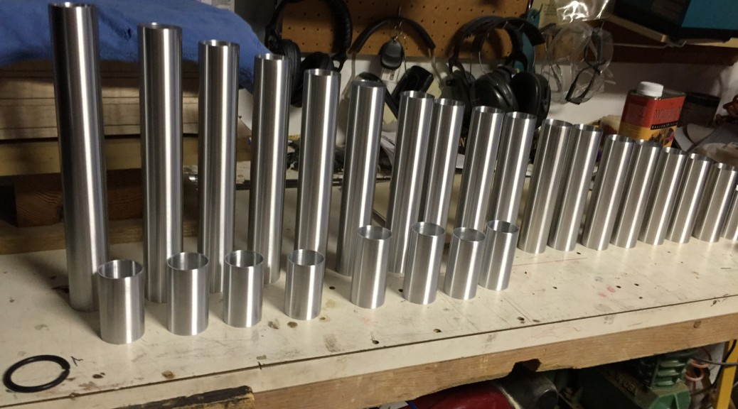
The resonator tubes are an important part of the xylophone. They boost and shape the sound produced by the bars. There is lots of information on the web about resonator tubes, so I won’t repeat that, but I will discuss our approach to making, mounting, and tuning the tubes.

The Physics

It is not hard to find info about “quarter wave stopped resonator tubes” on the web (in musical parlance these are sometimes called “stopped pipes.”) This is the type of resonator tube that is used for xylophones and marimbas These tubes basically resonate at a fundamental frequency of c/4L, where L is the length of the tube and c is the speed of sound. In simple terms, the tube boosts the bar sound amplitude by utilizing the normally wasted downward-directed sound energy in a way that boosts the upward facing energy (which is what you mostly hear). It shapes the sound too, because it does not boost all frequencies equally. In particular, it only boosts the fundamental and the odd harmonics. Because xylophone bars are tuned to a 1:3:6 frequency relationships, the fundamental and second partial will be boosted, but the third partial will not. This is another reason why I wasn’t too concerned about tuning the 3rd partial – its already puny energy is swamped by the boosted energy of the first two partials. Additionally, while we haven’t discussed it much, real xylophone bars “ring up” not just the “transverse modes” that dominate the sound, but also lesser “longitudinal” and “torsional” modes. Because these modes are not typically odd harmonics of the fundamental, they do not get amplified. So, at the end of the day, when tubes are added to the instrument, you mostly hear the fundamental and the second partial – all the other frequencies get dwarfed.

Tuning the tubes is done by adjusting a movable stopper that effectively changes the length of the tube. This is what determines the length L in the equation above. So you might think that tuning the tubes is just a matter of computing the tube length via the equation above and then setting the stopper to that length (I did,) however, like most equations from physics, the formula above is only approximate. It is very accurate under certain conditions, such as when the tube length to diameter ratio is large and the sound input to the tube is a “plane wave.” However, neither of these assumptions is true for the xylophone. In particular, the shorter tubes have a relatively low length-to-diameter ratio; and the sound wave coming off the bar is likely not planar, since the bottom of the bar is curved.

Dr Entwistle pointed me to a book called “The Physics of Musical Instruments,” by Rossing and Fletcher (ISBN-13: 978-1441931207,) that had some interesting comments about xylophones and ¼ wave resonators. In the section on resonator tubes, they note that the resonant frequency of the tube is a weak function of the distance between the tube end and the bottom of the bar. However, they state that “As yet, the theory describing the coupled bar-resonator system has not been worked out in detail,” which basically means that there is not a simple equation to compute the actual stopper position as a function of the desired frequency.

Additionally, the Rossing book describes a few topics of practical importance. First, the it describes something referred to as the “end correction factor.” It turns out that the equation above must be tweaked somewhat due to the fact that the standing wave in the tube does not end exactly at the pipe mouth but is rather a bit beyond it. The more accurate equation for the resonator frequency is f =c/[ 4(L+0.61r)], where r is the radius of the tube. I found other references to the end correction online and there appears to be some debate in the literature over the correct value of the correction factor (i.e., the value of 0.61).

As noted above, the book notes that the tube frequency is affected by the spacing between the tube end and the bar bottom. I had already seen that some xylophones allowed for adjustment of the height of the tube assembly (i.e., the assembly of all of the tubes locked together into a rigid structure) to compensate for temperature changes. It makes sense that if the tube-bar spacing is less than the 0.61r factor, then it will affect the tube resonance since the bar is effectively serving as a stop at the top of the tube.

At the end of the day, it became clear that the bars must be tuned in situ to obtain accurate tuning. However, I couldn’t resist the urge to check out the physics, so I did a few experiments and built some tuning curves that I hoped might at least guide the resonator tuning. However, in the spirit of full disclosure, I must note that I mostly ignored the results from this effort and just tuned the tubes by ear! Nevertheless, I will describe these experiments, if for no other reason than to perhaps save others the folly of this endeavor. You can safely skip this section without regret if you just want to git-er-done…

Tuning the Tubes

I started out by doing experiments with a piece of PVC as I awaited the delivery of the aluminum. I was particularly interested in verifying the resonant behavior of the tubes as a function of spacing distance to the bar. It wasn’t clear to me how to establish the correct tube-bar spacing. Intuitively, it seemed to me that the best coupling might result from close spacing, so that the spacing would be dictated by physical constraints, like avoiding contact if the bar should sag.

In order to start my experiments, I needed a value for the speed of sound. The speed of sound is a function of the density of the air, which is a function of the temperature. I found an online calculator here that computed the velocity. During my experiments, I measured the temperature at 19.2 C, and the the online calculator gave me a velocity of 343 m/s.

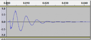
I must admit that I struggled a bit with how to find the resonant frequency for my PVC resonator pipe. I fabricated an adjustable stop and set it to yield a 15.0 cm tube. Per the standard 1/4 wave calculation (with a 0.61*r end correction,) the computed frequency was about 525 Hz. I experimented with several methods of exciting the bar. I tried whacking the end of the tube, and attempted to measure the impulse, but the resonance died out rather quickly. Here’s an example where you can see that the pulse dies out in about 25 ms:

I did some decayed sinusoidal fitting to this, but wasn’t able to get accurate results. Ultimately, I used a small speaker to excite the tube as shown in this photo:

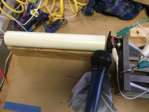
The tube was excited by the speaker at the right, and the resulting audio was recorded with the microphone.

Next, I tried exciting the tube with white noise. Interestingly, you could easily hear the “coloring” of the noise due to the modes. This gave PSD plots like this:

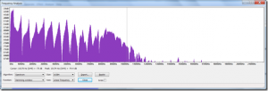
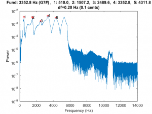
However, I found that identifying the peaks was unreliable. Ultimately, I wrote some Matlab code to generate and play a frequency sweep while recording the response. Here is an example of one of the PSD curves:

 

This is what the recording sounded like for this tube:

The code identifies the peaks (which of course correspond to odd harmonics). However, the first peak (the fundamental) was always a bit broad and had a sort of “shoulder” to it, which made me doubt it. So I wrote a little algorithm to find an the optimal “least common factor” for all of the identified peaks. The higher harmonics had generally broad peaks so I also ignored them, and only used the lower modes. In general the setup was somewhat fickle and the quality of the peaks that I got was a strong function of the microphone and speaker placement. In any case, here is some data for my 15 cm tube:

Temp = 19.2 deg C


>> ResonatorTune(500, 'res=15.0, spc=3.0')

res=15.0, spc=3.0 -

Fund: 509.0

, Error (Hz): 5.9, NumModes: 2

   Mode 1: Error (Hz): +10.6

   Mode 2: Error (Hz): -1.2

>> ResonatorTune(500, 'res=15.0, spc=2.0')

res=15.0, spc=2.0 -

Fund: 509.4

, Error (Hz): 6.0, NumModes: 2

   Mode 1: Error (Hz): +10.8

   Mode 2: Error (Hz): -1.3

>> ResonatorTune(500, 'res=15.0, spc=1.0')

res=15.0, spc=1.0 -

Fund: 505.0

, Error (Hz): 2.8, NumModes: 2

   Mode 1: Error (Hz): +5.0

   Mode 2: Error (Hz): -0.5

>> ResonatorTune(500, 'res=15.0, spc=0.5')

res=15.0, spc=0.5 -

Fund: 492.5

, Error (Hz): 3.4, NumModes: 2

   Mode 1: Error (Hz): +6.1

   Mode 2: Error (Hz): -0.7

These data correspond to 4 different collections with varying standoff distances from the end of the tube to the speaker (from 3.0 cm to 0.5 cm). It is interesting that the frequency doesn’t shift above about 2 cm, but there is a nearly 20 Hz shift when the tube is very close to the speaker. This clearly shows the behavior noted in the Rossing book (i.e., decreased frequency for close spacing,) which was pretty cool.

So using this technique, I set off to build a curve that could be used to set the stopper distance for each tube. I chose to set the distance at 0.5 cm, which is about as close as I could safely space the tubes from the bars without fear of contact. For each stopper distance, I performed a sweep and used my least-common-factor code to find the tube resonance. With this approach, I was able to build the following curve.

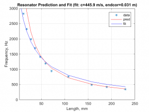
The blue points on the curve are the measurements and the red line was created using the frequency equation given above (including the 0.61r end correction factor). The equation accurately predicts the frequency for the longer pipes, but performs poorly for the short pipes. As a quick test, I tried fitting the equation above, but left the speed of sound and the end correction factor as free variables. This resulted in the blue curve. The fit was better for the short tubes, but resulted in poor performance for the long tubes. So I decided to skip function fitting entirely, and just set my stopper distances by interpolation between the measured points.

Next Up

This post described some of the science involved in establishing the tube resonant frequency. In the next post, I will describe the fabrication and mounting of the resonator tubes.