In the previous posts, I described the basic construction and tuning of a maple xylophone bar and promised that we would get into the woodworking next. However, we’ve got to do a bit more math first. Sorry for another bait-n-switch….

Rosewood Properties

As you may recall, the computer code that computes the bar shape requires the bulk modulus, shear modulus, and density to be specified. Apparently I am incapable of learning a lesson and again turned to the internet to provide these numbers. Like many of my previous attempts, I came up empty handed. Considering that all great Xylophones and Marimbas are made of one material – Honduras Rosewood – you might think that someone would have posted the material properties on the internet. If they did, Google and I couldn’t find it. This left me determined to compute them myself.

I did find a range of values for Young’s modulus (aka the bulk modulus) in a paper by Brémaud, et al. Figure 3a of the paper provided Young’s modulus values for  Honduras Rosewood (latin name Dalbergia Stevensonii) that span the range of 17-26 GPa. I am not sure why the range varied so much. Perhaps it is just natural variation in the wood? As an interesting aside, figure 3b of that same paper clearly shows that Honduras Rosewood has the lowest damping coefficient of all of the species evaluated, which the paper suggests is perhaps the most important quality for wood used to construct idiophones- this wood really is special.

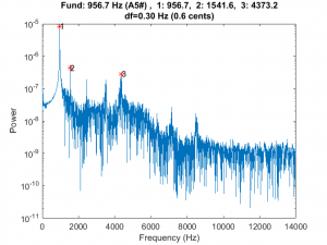
But the Zhao paper (and a few others that I found) came to the rescue. Appendix B of that paper, “Calculations for the Mechanical Properties,” provided a formula for calculating Young’s modulus from the fundamental frequency of a prismatic beam constructed from the material. My first job was to whack a Rosewood bar of known dimension and measure its fundamental. I had a couple of rosewood “test bars” that I cut to mess around with, and the longest one was 13-5/64 inches long. Here is the spectrum of that bar.

And here is the sound file for your listening pleasure.

From the spectrum, you can see that the fundamental was at about 957 Hz. You can check out the Zhao paper for the details of the equation, but here is the Matlab code to compute the modulus. (Note that the Zhao paper had an error in equation for E where beta_n should have been the constant beta_n*l)

inch2m=0.0254; %Conversion constant

%Compute the young's modulus from bar #1
b=1.501*inch2m; %width
h=0.880*inch2m; %height
L=(13+15/64)*inch2m; %Length

f1=957; %Measured frequency of fundamental
rho = 1082; %Density from measurement of volume and mass (see above)

A=b*h; %Cross sectional area
I=b*h^3/12; %Moment of inertial

E=4*pi^2*rho*A*L^4/I * (f1^2/4.73^4) %4.73 is a constant given by Zhao
%E = 2.396974370897572e+10

The modulus calculated for this bar was 23.9 GPa. I had a second bar that had a length of 9-27/64 inches and a fundamental frequency of 1867 Hz. The calculated modulus for this bar was 23.6 GPa – pretty close to the first number.

Zhao also gave a formula for the calculation of the shear modulus, G, but the torsional frequencies of the bar must be known. It was not clear to me that I could adequately “ring these up” and measure them, so getting the shear modulus using that approach seemed off the table. I decided to take a different tact.

My approach was to do a parametric sweep of the shear modulus using the Timoshenko code to compute the fundamental and first two overtones for a prismatic beam. My idea was that if I had the bulk modulus and density right (density was easy, I just weighed and measured the bar and divided the numbers,) then the only free variable was shear modulus. If I adjusted it until I made the Timoshenko-predicted frequencies match the measured frequencies, then I must have the right value for the shear modulus; right? Here are the results from that sweep for the long and short test bars.

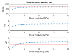
The red lines on the plots correspond to the measure modal frequencies based on my spectral measurements. This analysis was not entirely satisfying because the no value of G yielded the fundamental frequency – the prediction was always a bit lower than the measured value- however, inspection of the second and third partials suggested that a reasonable value for the shear modulus might be around 4 GPa.

For what it’s worth, I did find a published shear modulus value of 19 GPa for Padauk, a similar wood. This suggests my chosen value of 4 GPa might be too low, but I wasn’t sure what else to do – high values resulted in a very poor match for the overtones in the plots above. For what it’s worth, I computed some bar profiles with different values of G, and they didn’t vary a lot. So perhaps at the end of the day it’s not a big deal, since I knew I was going to have to “hand tune” the bars after roughly cutting to the computed shape anyway. Right or wrong, I forged on with my value of G=4 GPa.

Summary of Computed Results

With the Rosewood material properties estimated, I was able to run the minimizer/Timoshenko code to compute the bar profiles for each of my 44 rosewood bars. As I mentioned in a previous post, the minimizer is sensitive to the initial starting condition, so I seeded my first and longest bar, F4, with the cubic coefficients from the maple bar and watched the minimizer converge. For the rest of the bars, I initialized the minimizer by seeding it with the coefficients from the previous bar, working my way from longest to shortest. In this manor, I was able to leap-frog through the bars and ensure that the minimizer converged.

Here are some summary results from the computed bar runs. First, here are the fundamental frequencies as calculated by the Timoshenko and Euler methods for each of the bars.

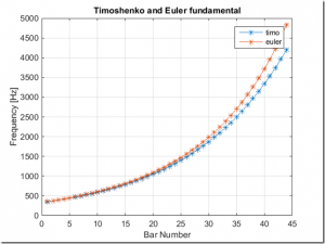
In every case, the code was able to perfectly converge to the desired fundamental frequency. The plot shows the results for the two methods. As previously noted, the Timoshenko method is generally more accurate, especially for the short bars.

Here are the ratios for the second and third overtones:

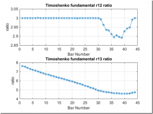
I found it interesting that the code can’t converge on the 2nd overtone for the short bars. No big deal because the overtones decay so rapidly for the shorter bars, it is doubtful that this effect can be heard. Indeed, when I was tuning the shorter bars, my spectral measurements were not able to measure the overtones.

The Templates Please

The computer run for each bar produces three standard plots. The first is the bar profile plot. An example for bar 10 is shown here.

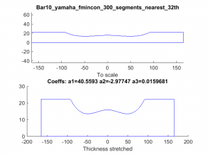
You’ve see plots like this before. The top figure has a 1:1 aspect ratio and gives an idea of the actual physical profile of the bar. The bottom figure has a arbitrary aspect ratio to better visualize the shape of the undercut. Also included on the figure are the coefficients for the cubic function that describes the profile curve. I followed Dr Entwistle’s definition for the cubic coefficients where

y=a1*x^3 + a2*x^2 + a3;

In this equation, x is the longitudinal length down the bar where x=0 is the bar center. The variable y denotes the bar thickness corresponding to each value of x. Notice that when x=0, the equation reduces to y=a3, which is the thickness at the center. Also, notice that there is no linear term with x (i.e., no coefficient that multiples x). Setting the linear coefficient to zero forces the cubic function to have zero a slope at x=0. This forces symmetry about the bar middle.

Note that there is nothing magical about using a cubic to represent the bar shape. Indeed, if I were going to build another xylophone, I might mess around with other functional forms to see if I could satisfy additional constraints, like forcing the third partial ratio to be 6.0, or to maximize sustain or volume. However, the cubic is a good compromise in that does a respectable job of providing shapes that mimic what I had seen on other xylophones while keeping the degrees of freedom low (i.e., just 3 coefficients).

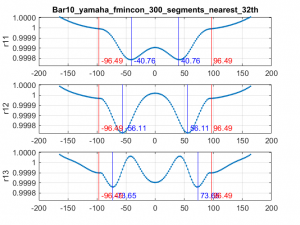
The second standard plot that I compute is the tuning curve, which we have discussed at length. For completeness, here is the tuning curve for my #10 bar.

Finally, as described in the maple bar fabrication discussion, I create a full-size paper template for each bar. Here is the template for bar #10:

A couple of notes about the annotations on this template are in order. The two vertical red lines mark the node locations as computed by the Euler code provided by Dr Entwistle. These are where the holes will be drilled. The vertical blue lines, marked f1, f2 and f3 denote fiducials on the bar corresponding to the tuning curve peaks. The f1 mark denotes the location where the fundamental is most affected by wood removal. Similarly, f2 marks the location where wood removal most dramatically changes the second partial, and f3 corresponds to the most sensitive region for the third partial.

All of these are useful plots, so I have zipped up the three curves for each of the 44 bars into a single file for you to download…I am just that kind of a guy 🙂

Here is the zip file: standard_plots_for_all_44_bars

Note that each of the files is a PDF, including the bar templates. The templates’ PDF files have been created so that they should print full-size. I made these to print on 8.5 x 14 inch paper, which was the largest size that my printer would handle. I am not sure how they will print on a smaller page size, but in any case, you should be able to scale these based on the bar sizes that I provided in the Excel file in the previous post.

In the next post we will actually start cutting Rosewood. (I know, you’ve heard that before. But you didn’t think you could build a xylophone without math, did you?)

 

References

Iris Brémaud, Pierre Cabrolier, Kazuya Minato, Jean Gérard, Bernard Thibaut. Vibrational properties of tropical woods with historical uses in musical instruments. Joseph Gril.International Conference of COST Action IE0601 Wood Science for the Preservation of Cultural Heritage, Nov 2008, Braga, Portugal. pp.17-23, 2010. <hal-00808403>